A seasonal SIR metapopulation model with an Allee effect with application to controlling plague in prairie dog colonies

Figures & data

Figure 1. Example curve ${\mathcal{B}}_i(N_i)$ satisfying assumption $\mathcal{A}2$.

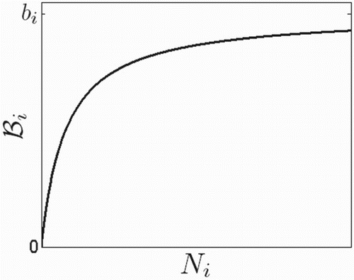
Figure 2. Function ${\phi }_{U_1}(t)$.

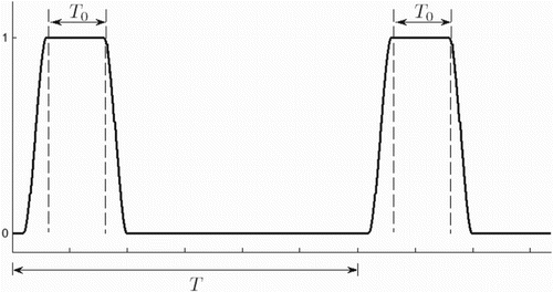
Table 1. Transitions $\mathrm{\Delta }\mathit{X}(t)=\mathit{X}(t+\mathrm{\Delta }t)-\mathit{X}(t)$, and the respective values $p(\mathrm{\Delta }\mathit{X}(t))=(1/\mathrm{\Delta }t)\mathrm{Prob}\{\mathrm{\Delta }\mathit{X}(t)|\mathit{X}(t)\}$, where vector ${\mathit{e}}_{X_i}$ has unity in the position corresponding to a variable $X_i$ and zeros elsewhere.

$\mathrm{\Delta }\mathit{X}$	$p(\mathrm{\Delta }\mathit{X})$	$\mathrm{\Delta }\mathit{X}$	$p(\mathrm{\Delta }\mathit{X})$
${\mathit{e}}_{S_i}$	${\phi }_{U_1}(t){\mathcal{B}}_i(N_i)N_i$	${\mathit{e}}_{I_i}-{\mathit{e}}_{S_i}$	${\beta }_i{S}_i{I}_i+\rho (S_i)\sum _{k=1}^K\sum _{l=1}^{L_k}{\beta }_i^{(kl)}{Y}_i^{(kl)}$
$-{\mathit{e}}_{S_i}$	$(d_i+c_i{N}_i)S_i$	${\mathit{e}}_{R_i}-{\mathit{e}}_{S_i}$	$v_i{S}_i$
$-{\mathit{e}}_{I_i}$	$(d_i^I+c_i{N}_i)I_i$	${\mathit{e}}_{Z_i^{(k)}}$	${\phi }_{U_3^{(k)}}(t){\mathcal{B}}^{(k)}(N_i,N_i^{(k)})N_i^{(k)}$
$-{\mathit{e}}_{R_i}$	$(d_i+c_i{N}_i)R_i$	$-{\mathit{e}}_{Z_i^{(k)}}$	$d_i^{(k)}{Z}_i^{(k)}$
${\mathit{e}}_{S_i}-{\mathit{e}}_{I_i}$	${\alpha }_1{\gamma }_i{I}_i$	$-{\mathit{e}}_{Y_i^{(kl)}}$	$d_i^{(kl)}{Y}_i^{(kl)}$
${\mathit{e}}_{R_i}-{\mathit{e}}_{I_i}$	$(1-{\alpha }_1){\gamma }_i{I}_i$	${\mathit{e}}_{Y_i^{(kl)}}-{\mathit{e}}_{Z_i^{(k)}}$	${\lambda }_i^{(kl)}\rho (I_i)Z_i^{(kl)}$
${\mathit{e}}_{S_i}-{\mathit{e}}_{S_j}$	${\phi }_{U_2}(t)m_{ij}{S}_j$	${\mathit{e}}_{Z_i^{(k)}}-{\mathit{e}}_{Y_i^{(kl)}}$	${\gamma }_i^{(kl)}h(S_i,I_i,R_i)Y_i^{(kl)}$
${\mathit{e}}_{I_i}-{\mathit{e}}_{I_j}$	${\phi }_{U_2}(t)m_{ij}^I{I}_j$	${\mathit{e}}_{Z_i^{(k)}}-{\mathit{e}}_{Z_j^{(k)}}$	${\phi }_{U_4^{(k)}}(t)m_{ij}^{(k)}\rho (S_j+R_j)Z_j^{(k)}$
${\mathit{e}}_{R_i}-{\mathit{e}}_{R_j}$	${\phi }_{U_2}(t)m_{ij}{R}_j$	${\mathit{e}}_{Y_i^{(kl)}}-{\mathit{e}}_{Y_j^{(kl)}}$	${\phi }_{U_4^{(k)}}(t)m_{ij}^{(kl)}\rho (I_j)Y_j^{(kl)}$

It is assumed that $\mathrm{\Delta }t>0$ is sufficiently small so that $\mathrm{Prob}\{\mathrm{\Delta }\mathit{X}=\mathbf{0}|\mathit{X}(t)\}=\alpha >0$, with α equalling the difference between unity and the sum of all probabilities $\mathrm{Prob}\{\mathrm{\Delta }\mathit{X}(t)|\mathit{X}(t)\}=\mathrm{\Delta }tp(\mathrm{\Delta }X(t))$ for all listed values $p(\mathrm{\Delta }\mathit{X})$ and all appropriate values of $i,j,k,l$:$i,j=1,\dots ,p$, $l=1,\dots ,L_k$, $k=1,\dots ,K$.

Table 2. List of variables within patch i, $i=1,\dots ,p$.

Variable	Description
$S_i$	Susceptible hosts (C. ludovicianus)
$I_i$	Infectious hosts
$R_i$	Immune hosts
$N_i$	$S_i+I_i+R_i$
$Z_i^{\mathrm{h}}$	Susceptible O. hirsuta
$Y_i^{\mathrm{h}}$	Infectious unblocked O. hirsuta
$Y_i^{\mathrm{hB}}$	Infectious blocked O. hirsuta
$N_i^{\mathrm{h}}$	$Z_i^{\mathrm{h}}+Y_i^{\mathrm{t}}+Y_i^{\mathrm{tB}}$
$Z_i^{\mathrm{t}}$	Susceptible O. t. cynomuris
$Y_i^{\mathrm{t}}$	Infectious O. t. cynomuris (unblocked)
$N_i^{\mathrm{t}}$	$Z_i^{\mathrm{t}}+Y_i^{\mathrm{h}}$

Figure 3. Flea parameters $b^{\mathrm{h}}$, $b^{\mathrm{t}}$, and $d^{\mathrm{t}}$ were obtained by fitting Equations (10$\begin{array}{rl}\frac{\mathrm{d}{Z}_i^{\mathrm{h}}}{\mathrm{d}t}& ={\phi }_{U_3^{\mathrm{h}}}(t)\left(\frac{b^{\mathrm{h}}{N}_i}{1+N_i+N_i^{\mathrm{h}}}\right)N_i^{\mathrm{h}}-\left(d_i^{\mathrm{h}}+{\lambda }^{\mathrm{h}}\left(\frac{I_i}{N_i+1}\right)\right)Z_i^{\mathrm{h}}+{\gamma }^{\mathrm{h}}\left(\frac{S_i+R_i}{N_i+1}\right)Y_i^{\mathrm{h}}\\ & +\sum _{j=1}^p\frac{m}{x_{ij}}\left[\left(\frac{S_j+R_j}{N_j+1}\right)\frac{Z_j^{\mathrm{h}}}{A_j}-\left(\frac{S_i+R_i}{N_i+1}\right)\frac{Z_i^{\mathrm{h}}}{A_i}\right],\\ \frac{\mathrm{d}{Y}_i^{\mathrm{h}}}{\mathrm{d}t}& ={\alpha }_2{\lambda }^{\mathrm{h}}\left(\frac{I_i}{N_i+1}\right)Z_i^{\mathrm{h}}-\left(d_i^{\mathrm{hU}}+{\gamma }^{\mathrm{h}}\left(\frac{S_i+R_i}{N_i+1}\right)\right)Y_i^{\mathrm{h}}\\ & +\sum _{j=1}^p\frac{m^I}{x_{ij}}\left[\left(\frac{I_j}{N_j+1}\right)\frac{Y_j^{\mathrm{h}}}{A_j}-\left(\frac{I_i}{N_i+1}\right)\frac{Y_i^{\mathrm{h}}}{A_i}\right],\\ \frac{\mathrm{d}{Y}_i^{\mathrm{tB}}}{\mathrm{d}t}& =(1-{\alpha }_2){\lambda }^{\mathrm{h}}\left(\frac{I_i}{N_i+1}\right)Z_i^{\mathrm{h}}-d_i^{\mathrm{hB}}{Y}_i^{\mathrm{hB}},\end{array}$) and (11$\begin{array}{rl}\frac{\mathrm{d}{Z}_i^{\mathrm{t}}}{\mathrm{d}t}& ={\phi }_{U_3^{\mathrm{t}}}(t)\left(\frac{b^{\mathrm{t}}{N}_i}{1+N_i+N_i^{\mathrm{t}}}\right)N_i^{\mathrm{t}}-\left(d_i^{\mathrm{t}}+{\lambda }^{\mathrm{t}}\left(\frac{I_i}{N_i+1}\right)\right)Z_i^{\mathrm{t}}+{\gamma }^{\mathrm{t}}\left(\frac{S_i+R_i}{N_i+1}\right)Y_i^{\mathrm{t}}\\ & +\sum _{j=1}^p\frac{m}{x_{ij}}\left[\left(\frac{S_j+R_j}{N_j+1}\right)\frac{Z_j^{\mathrm{t}}}{A_j}-\left(\frac{S_i+R_i}{N_i+1}\right)\frac{Z_i^{\mathrm{t}}}{A_i}\right],\\ \frac{\mathrm{d}{Y}_i^{\mathrm{t}}}{\mathrm{d}t}& ={\lambda }^{\mathrm{t}}\left(\frac{I_i}{N_i+1}\right)Z_i^{\mathrm{t}}-\left(d_i^{\mathrm{tU}}+{\gamma }^{\mathrm{t}}\left(\frac{S_i+R_i}{N_i+1}\right)\right)Y_i^{\mathrm{t}}\\ & +\sum _{j=1}^p\frac{m^I}{x_{ij}}\left[\left(\frac{I_j}{N_j+1}\right)\frac{Y_j^{\mathrm{t}}}{A_j}-\left(\frac{I_i}{N_i+1}\right)\frac{Y_i^{\mathrm{t}}}{A_i}\right],\end{array}$), in the absence of infection and migration, to monthly flea load data (marked by +), given in [78].

Table 3. Rate values for calculating ${\beta }^{\mathrm{h}}$ and ${\beta }^{\mathrm{t}}$.

Parameter	O. hirsuta	O. t. cynomuris
Vector efficiency	0.045	0.18
Daily biting rate	0.84	0.82
Unblocked transmission	${\beta }^{\mathrm{h}}=0.006$	${\beta }^{\mathrm{t}}=0.025$

Note: Related reference: [78].

Table 4. Prairie dog parameter values (per year, except for $d_i^I$, which is given per day^*).

Parameter	Value		Description	Reference
b	0.434		Birth parameter,	Calculated,
			$U_1$: Mar–Apr	[40, 41, 44, 48, 72]
$d_i$	0.274	$\mathrm{\forall }i$	Natural mortality	Calculated, [78]
$d_i^I$	0.167^*	$\mathrm{\forall }i$	Infectious mortality	[14, 18, 44]
c	$1.78\times {10}^{-2}$		Crowding	Calculated, [72]
m	$4\times {10}^{-3}$		Migration parameter,	Assumed
			$U_2$: Apr–May
$m^I$	$4\times {10}^{-5}$		Infectious migration parameter	Assumed

Table 5. Flea parameter values (per day).

Parameter	Value		Description	Reference
${\beta }^{\mathrm{h}}$	$6\times {10}^{-3}$		Transmission coefficient	Table 3
${\beta }^{\mathrm{hB}}$	$1\times {10}^{-3}$		Transmission coefficient	Calculated [18, 28, 78]
${\beta }^{\mathrm{t}}$	$2.5\times {10}^{-2}$		Transmission coefficient	Table 3
$b^{\mathrm{h}}$	0.25		Birth parameter,	Figure 3
			$U_3^{\mathrm{h}}$: mid-Apr–mid-Dec
$b^{\mathrm{t}}$	0.55		Birth parameter,	Figure 3
			$U_3^{\mathrm{t}}$: mid-Jan–mid-Mar
$d_i^{\mathrm{h}}$	$1.667\times {10}^{-2}$	$\mathrm{\forall }i$	Natural mortality	Figure 3
$d_i^{\mathrm{t}}$	$3.333\times {10}^{-2}$	$\mathrm{\forall }i$	Natural mortality	Figure 3
$d_i^{\mathrm{hU}}$	0.05	$\mathrm{\forall }i$	Post-infection mortality	[78]
$d_i^{\mathrm{tU}}$	0.12	$\mathrm{\forall }i$	Post-infection mortality	[78]
$d_i^{\mathrm{hB}}$	0.06	$\mathrm{\forall }i$	Blocked mortality	Calculated with 2 weeks incubation [18, 28, 55]
${\lambda }^{\mathrm{h}}$	1		Infection prevalence	[78]
${\lambda }^{\mathrm{t}}$	0.88		Infection prevalence	[78]
${\gamma }^{\mathrm{h}}$	0.2		Recovery	Assumed
${\gamma }^{\mathrm{t}}$	0.2		Recovery	Assumed

Note: Superscripts h and t correspond to species O. hirsuta and O. t. cynomuris, respectively.

Figure 4. Function ${\sigma }_0=\sigma (\mathrm{diag}({\tilde{\phi }}_{U_1}b/k{A}_i-d_i)+\frac{1}{2}{\tilde{\phi }}_{U_2}(\mathbf{M}+{\mathbf{M}}^{\mathrm{T}}))$ for various values of k, where $\sigma (\mathbf{A})$ denotes the largest eigenvalue of a symmetric matrix $\mathit{A}$ and k is the parameter in the birth rate ${\mathcal{B}}_i(N_i)$ which controls the level of the Allee effect. A strong Allee effect exists when ${\sigma }_0<0$.

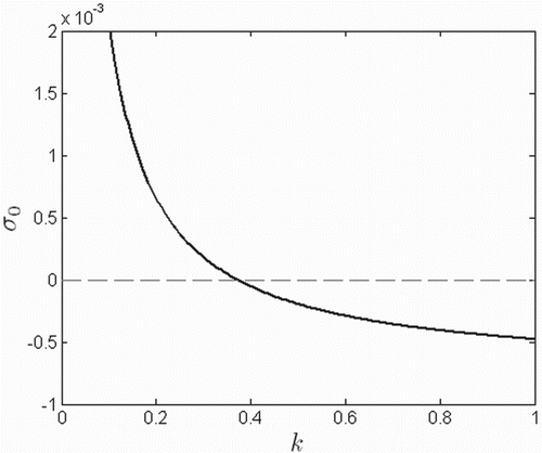
Figure 5. Population size over five years in the absence of disease for the smallest patch ($i=6$, left) and the largest patch ($i=2$, right), for $k=0.1,0.3,0.5,$ and 0.7, according to the ODE model. Time t is given in days. A strong Allee effect is evident for values of k such that ${\sigma }_0<0$.

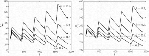
Figure 6. Seventy-year ODE solution curves for Rankin Ridge, $N_6(t)$, in the absence of infection, with the initial conditions $N_i(t_0)=1.2A_i,1.7A_i,$ and $10A_i$ for all i, where $A_i$ is the area of patch i. Time t is given in days and $t_0$ is the beginning of the prairie dog birth season. Solutions approach a positive periodic solution for initial conditions exceeding periodic threshold $x_i(t)$ for all i.

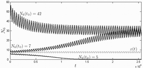
Figure 7. Five-year solution curves for prairie dog classes $S_i(t)$ and $I_i(t)$ for three patches ($i=11,$ 7, and 2, north to south from left to right) and for unblocked flea proportions ${\alpha }_2=0$ (top row), 0.5 (second row), and 1 (third row), based on the ODE model (dark) and one sample path of the SDE model (light) for the initial conditions given in Equation (12$\begin{array}{r}\begin{array}{rl}{I}_i(0)& =0,Y_i^{\mathrm{h}}(0)=0,Y_i^{\mathrm{hB}}=0,Y_i^{\mathrm{t}}(0)=0,i=1,\dots ,11,\\ N_i(0)& =5A_i,N_i^{\mathrm{h}}(0)=0.675N_i(0),N_i^{\mathrm{t}}(0)=0,i=1,\dots ,11,\end{array}\end{array}$), and introducing two infected prairie dogs in North Boundary on day 120:$I_{11}(120)=2$. For this example, only O. hirsuta is modelled, without O. t. cynomuris. Blocked individuals are not as effective at transmitting plague as unblocked.

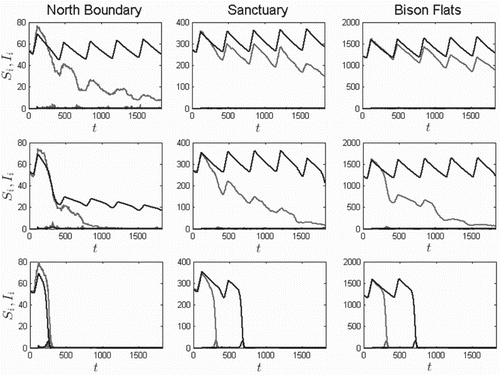
Figure 8. Two-year solution curves for three patches (north to south from left to right, $i=11,$ 7, and 2, respectively) for the two-flea species model and ${\alpha }_2=1$ (no blocked O. hirsuta), based on the ODE model (dark) and one sample path of the SDE model (light) for the initial conditions given in Equation (13$\begin{array}{r}\begin{array}{rl}{I}_i(0)& =0,Y_i^{\mathrm{h}}(0)=0,Y_i^{\mathrm{t}}(0)=0,i=1,\dots ,11,\\ N_i(0)& =5A_i,N_i^{\mathrm{h}}(0)=0.675N_i(0),N_i^{\mathrm{t}}(0)=0.0005N_i(0),i=1,\dots ,11,\end{array}\end{array}$). As in Figure 7, two infectious prairie dogs are introduced into North Boundary at time 120 days: $I_{11}(120)=2$. The models predict a much faster spread of plague with both species included.

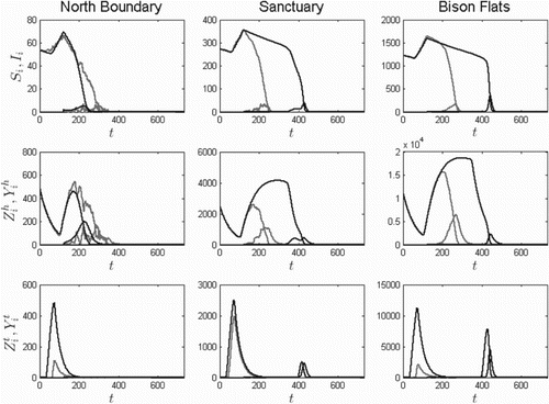
Figure 9. Time (in days) to extinction of each patch for the ODE model (connected circles) and 1000 sample paths of the SDE model (box plots), using initial conditions given by Equation (13$\begin{array}{r}\begin{array}{rl}{I}_i(0)& =0,Y_i^{\mathrm{h}}(0)=0,Y_i^{\mathrm{t}}(0)=0,i=1,\dots ,11,\\ N_i(0)& =5A_i,N_i^{\mathrm{h}}(0)=0.675N_i(0),N_i^{\mathrm{t}}(0)=0.0005N_i(0),i=1,\dots ,11,\end{array}\end{array}$) and introducing $I_{11}(120)=2$. Patches are ordered by distance from North Boundary, from closest (left, North Boundary itself) to furthest (right). See Figure A1 and Table A2 for the spatial arrangement. The ODE model predicts much longer times to extinction for every patch except North Boundary.

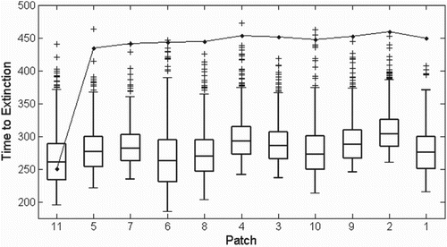
Figure 10. Five-year numerical solutions for prairie dog and flea populations in North Boundary ($i=11$) for control (insecticide) -induced death rates resulting in 75%, 85%, and 95% death at the end of the application compared to levels immediately prior to application, based on the ODE model (dark) and one realization of the SDE model (light). Time t is in days, initial conditions are given by Equation (13$\begin{array}{r}\begin{array}{rl}{I}_i(0)& =0,Y_i^{\mathrm{h}}(0)=0,Y_i^{\mathrm{t}}(0)=0,i=1,\dots ,11,\\ N_i(0)& =5A_i,N_i^{\mathrm{h}}(0)=0.675N_i(0),N_i^{\mathrm{t}}(0)=0.0005N_i(0),i=1,\dots ,11,\end{array}\end{array}$), and $I_{11}(120)=2$. Insecticide is ineffective at 75%, controls the population at 85%, and prevents plague-driven decline in the prairie dog population at 95%.

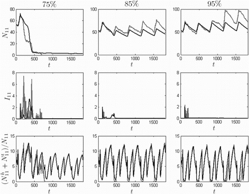
Figure 11. Twenty-year solutions $N_{11}$ with (bottom) and without (top) the Allee effect, for vector control using death rates resulting in 75% death at the end of the application compared to levels immediately prior to application, based on the ODE model (dark) and one realization of the SDE model (light). Time t is in days, initial conditions are given by Equation (13$\begin{array}{r}\begin{array}{rl}{I}_i(0)& =0,Y_i^{\mathrm{h}}(0)=0,Y_i^{\mathrm{t}}(0)=0,i=1,\dots ,11,\\ N_i(0)& =5A_i,N_i^{\mathrm{h}}(0)=0.675N_i(0),N_i^{\mathrm{t}}(0)=0.0005N_i(0),i=1,\dots ,11,\end{array}\end{array}$), and $I_{11}(120)=2$. In the absence of the Allee effect, the model predicts eventual recovery of the prairie dog population under this level of vector control, whereas with the Allee effect, the population faces extinction.

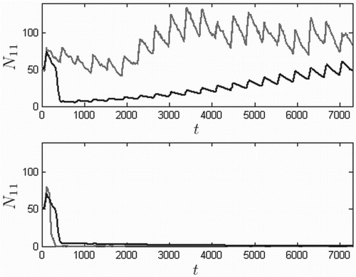
Figure 12. Ten-year North Boundary ($i=11$) solution curves $N(t)$, $I(t)$, and $R(t)$ for annual vaccination from May through July, at rates that result in 10% (left), 20% (middle), and 30% (right) vaccinated by the end vaccination period, for the ODE model (dark) and one sample path of the SDE model (light). Time t is in days, initial conditions are given by Equation (13$\begin{array}{r}\begin{array}{rl}{I}_i(0)& =0,Y_i^{\mathrm{h}}(0)=0,Y_i^{\mathrm{t}}(0)=0,i=1,\dots ,11,\\ N_i(0)& =5A_i,N_i^{\mathrm{h}}(0)=0.675N_i(0),N_i^{\mathrm{t}}(0)=0.0005N_i(0),i=1,\dots ,11,\end{array}\end{array}$), and $I_{11}(120)=2$. Although the plague suppresses the population, the patch avoids extinction when vaccination rates are sufficiently high.

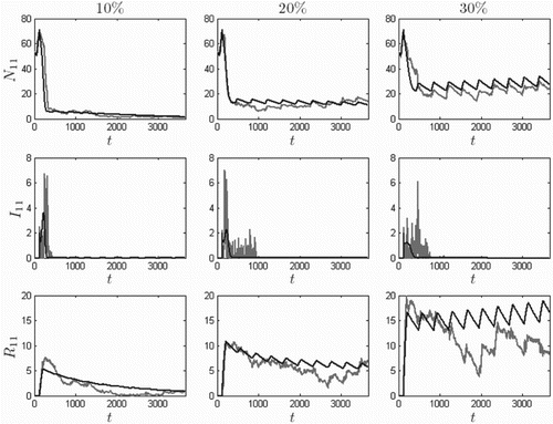
Figure A1. Prairie dog town locations with respect to one another. Related references: [19, 65].

Table A1. Area occupied by prairie dog colonies in Wind Cave National Park, South Dakota.

Number	Name	Area $(\mathrm{in}{10}^4{\mathrm{m}}^2)$
1	Shirttail	14.1
2	Bison Flats	246.4
3	Norbeck	62.5
4	Research Reserve	108.7
5	Pringle	29.0
6	Rankin Ridge	4.2
7	Sanctuary	54.8
8	Highland	12.2
9	Southeast	59.4
10	Northeast	13.8
11	North Boundary	10.7

Related reference: [19].

Table A2. Distances (in 10³m) between closest edges of prairie dog colonies in Wind Cave National Park, South Dakota. Colony names and corresponding patch numbers are given in Table A1.

Colony	1	2	3	4	5	6	7	8	9	10	11
1	0	0.80	4.02	4.83	9.12	9.12	8.85	10.73	9.66	16.09	11.80
2	0.80	0	1.88	2.14	7.77	7.51	6.44	6.97	5.90	11.80	9.66
3	4.02	1.88	0	0.72	4.56	4.56	4.02	5.63	6.44	11.67	6.71
4	4.83	2.14	0.72	0	4.83	4.30	3.09	3.76	4.02	9.66	6.17
5	9.12	7.77	4.56	4.83	0	1.08	1.61	5.63	9.12	11.14	1.07
6	9.12	7.51	4.56	4.30	1.08	0	1.48	5.10	8.32	10.99	2.06
7	8.85	6.44	4.02	3.09	1.61	1.48	0	2.82	6.17	8.85	1.34
8	10.73	6.97	5.63	3.76	5.63	5.10	2.82	0	3.22	5.63	4.56
9	9.66	5.90	6.44	4.02	9.12	8.32	6.17	3.22	0	5.90	8.58
10	16.09	11.80	11.67	9.66	11.14	10.99	8.85	5.63	5.90	0	8.32
11	11.80	9.66	6.71	6.17	1.07	2.06	1.34	4.56	8.58	8.32	0

Related references: [19, 65].

A.P. Wilder, R.J. Eisen, S.W. Bearden, J.A. Montenieri, D.W. Tripp, R.J. Brinkerhoff, K.L. Gage, and M.F. Antolin, Transmission efficiency of two flea species (oropsylla tuberculata cynomuris and oropsylla hirsuta) involved in plague epizootics among prairie dogs, EcoHealth 5 (2008), pp. 205–212. doi: 10.1007/s10393-008-0165-1

 PubMed Web of Science ®Google Scholar

J.L. Hoogland, Black-tailed, Gunnison's, and Utah prairie dogs reproduce slowly, J. Mammal. 82 (2001), pp. 917–927. doi: 10.1644/1545-1542(2001)082<0917:BTGSAU>2.0.CO;2

 Web of Science ®Google Scholar

J.L. Hoogland, D.K. Angell, J.G. Daley, and M.C. Radcliffe, Demography and population dynamics of prairie dogs, Great Plains Wildlife Damage Control Workshop Proceedings, 1987. Available at http://digitalcommons.unl.edu/gpwdcwp/72.

 Google Scholar

P. Johnsgard, Prairie Dog Empire: A Saga of the Shortgrass Prairie, University of Nebraska Press, Lincoln, NE, 2005.

 Google Scholar

C.B. Koford, Prairie dogs, whitefaces, and blue grama, Wildlife Monographs no. 3, p. 78.

 Google Scholar

E. Ulev, Cynomys ludovicianus. Fire effects information system [online]. U.S. Department of Agriculture, Forest Service, Rocky Mountain Research Station, Fire Sciences Laboratory (producer), 2007. Last accessed August 2, 2013. Available at http://www.fs.fed.us/database/feis/.

 Google Scholar

S.K. Collinge, W.C. Johnson, C. Ray, R. Matchett, J. Grensten, J.F. Cully Jr., K.L. Gage, M.Y. Kosoy, J.E. Loye, and A.P. Martin, Landscape structure and plague occurrence in black-tailed prairie dogs on grasslands of the western USA, Landscape Ecol. 20 (2005), pp. 941–955. doi: 10.1007/s10980-005-4617-5

 Web of Science ®Google Scholar

J.F. Cully Jr. and E.S. Williams, Interspecific comparisons of sylvatic plague in prairie dogs, J. Mammal. 82 (2001), pp. 894–905. doi: 10.1644/1545-1542(2001)082<0894:ICOSPI>2.0.CO;2

 Web of Science ®Google Scholar

C.R. Eskey and V. Haas, Plague in the western part of the United States: Infection in rodents, experimental transmission by fleas, and inoculation tests for infection, Public Health Rep. 54(32) (1939), pp. 1467–1481. doi: 10.2307/4582984

 PubMedGoogle Scholar

E.A. Lorange, B.L. Race, F. Sebbane, and B.J. Hinnebusch, Poor vector competence of fleas and the evolution of hypervirulence in Yersinia pestis, J. Infect. Dis. 191 (2005), pp. 1907–1912. doi: 10.1086/429931

 PubMed Web of Science ®Google Scholar

K. Dalsted, S. Sather-Blair, B. Worcester, and R. Klukas, Application of remote sensing to prairie dog management, J. Range Manage. 34(3) (1981), pp. 218–223. doi: 10.2307/3898046

 Google Scholar

Prairie dog towns 2003, Resource Ramblings 2004-05, Wind Cave National Park Management News Briefs, National Park Service. Last accessed March 1, 2014. Available at http://www.nps.gov/wica/naturescience/resource-ramblings-2004-05.htm.

 Google Scholar