Bootstrapping least-squares estimates in biochemical reaction networks

Figures & data

Table 1. Penalized vs. ordinary LSEs for L1.

			LSE		PLSE
Coefficient	n	${\gamma }_n$	Mean	Variance	Mean	Variance
${\beta }_1=5$	10	0.18	5.84	55.54	3.95	5.51
${\beta }_2=1$			1.82	47.27	0.96	10.05
${\beta }_3=0.1$			0.10	0.0115	0.13	0.0049
${\beta }_1=5$	100	0.032	5.16	4.09	4.74	2.24
${\beta }_2=1$			1.02	4.18	0.94	3.56
${\beta }_3=0.1$			0.10	0.0013	0.11	0.0010
${\beta }_1=5$	1000	0.0056	5.04	1.18	4.95	1.01
${\beta }_2=1$			0.99	0.67	0.97	0.66
${\beta }_3=0.1$			0.10	0.0005	0.10	0.0004
${\beta }_1=5$	10,000	0.001	5.02	0.89	5.00	0.88
${\beta }_2=1$			1.00	0.25	0.99	0.25
${\beta }_3=0.1$			0.10	0.0003	0.10	0.0004

The comparison of the lasso-penalized and the ordinary LSE estimates in terms of their mean and variance illustrates the reduction in variation due to the presence of penalty term. For smaller system sizes the advantage of the penalized estimates for variance reduction are especially apparent.

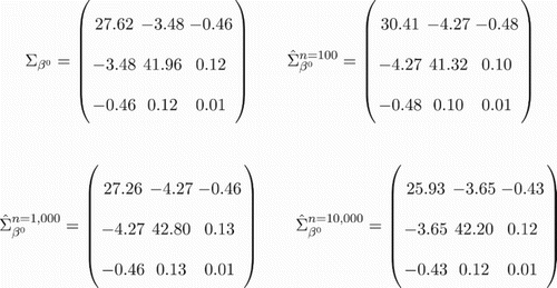
Figure 1. Bootstrap estimate of the LSE covariance for the L1 system. True asymptotic LSE covariance matrix vs. diffusion bootstrap covariance matrices for L1 systems with varying n (via Algorithm 1). To facilitate comparisons, the penalty was removed, i.e. ${\gamma }_n=0$ for all cases considered.

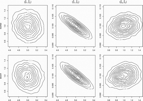
Figure 2. LSE covariance recovery via bootstrap for the L1 system. The contour plots for the true asymptotic LSE bivariate marginal distributions (top panel) and their LNA bootstrap estimates (bottom panel) for the LSE in the L1 system with $n=1000$. The recovery of the multivariate Gaussian distribution covariance structure by the bootstrap procedure is clearly visible.

Table 2. Time-course RT-PCR experiment results for L1 gene.

Time (h)	0.16	0.5	1	3	12	24	48	72	96
L1 Rel. Con.	12.583	14.459	12.183	11.985	13.295	12.168	9.584	9.841	6.298

Figure 3. Bootstrap likelihood profiling. The LNA bootstrap ($M=5000$) plots approximating for several different n values the residuals distributions for the model (18(18) $c_1^{\beta }\left(t\right)={\beta }_1{\beta }_3[1+(1+t{\beta }_2\left){\mathrm{e}}^{-{\beta }_{2}t}\right].$(18) ) fitted to data in Table 2 and comparing them with the actual observed residuals (grey vertical lines). As seen from the plots, around the value $n=5000$ the mode of the residuals distribution best aligns with the observed value. Note that the alignment is very poor for $n=1000$, which is the estimated volume used in [16].

Figure 4. Confidence envelopes for different n values. The ODE model data (18(18) $c_1^{\beta }\left(t\right)={\beta }_1{\beta }_3[1+(1+t{\beta }_2\left){\mathrm{e}}^{-{\beta }_{2}t}\right].$(18) ) fitted to the trajectory data in Table 2 plotted along with the fits 95% confidence envelopes for two different estimated system sizes. The left panel shows the bounds obtained in [16] for the system size $n=1000$ whereas the right panel shows the bounds obtained by taking $n=5000$.

G.A. Rempala, Least squares estimation in stochastic biochemical networks, Bull. Math. Biol. 74(8) (2012), pp. 1938–1955. doi: 10.1007/s11538-012-9744-y

 PubMed Web of Science ®Google Scholar