
Figures & data
Figure 1. The data sets of interest from [Citation9,Citation25]. The total polymerized mass is measured by Thioflavin T (ThT), which is one of the most common experimental tools for in vitro protein polymerization [Citation25,Citation29]. (available in colour online)
![Figure 1. The data sets of interest from [Citation9,Citation25]. The total polymerized mass is measured by Thioflavin T (ThT), which is one of the most common experimental tools for in vitro protein polymerization [Citation25,Citation29]. (available in colour online)](/cms/asset/9e065c6a-b2d5-4983-ac1f-8a0ef4d0931f/tjbd_a_1050465_f0001_c.jpg)
Figure 2. Parametric representation for .
Figure 3. Plots with simulated data: (a) correct cost function vs. time ; (b) incorrect cost function vs. time
.
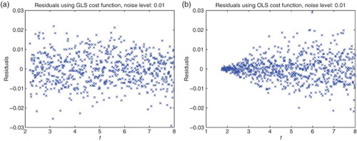
Figure 4. Plots with simulated data: (a) correct cost function vs. model ; (b) incorrect cost function vs. model
.
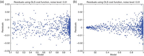
Figure 5. (a) (Madim) with OLS; (b) residuals vs. model: OLS.
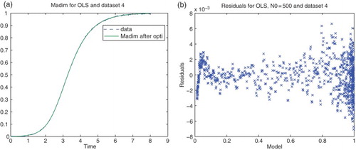
Figure 6. (a) with GLS,
; (b) residuals vs. model: GLS.
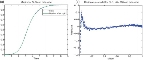
Figure 7. Residuals for DS4 using different values of γ.
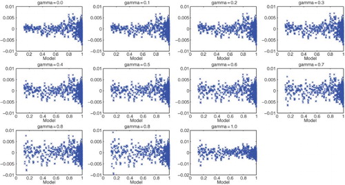
Figure 8. Residuals for the four experimental data sets using .
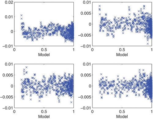
Figure 9. (a) Sensitivity w.r.t. ; (b) sensitivity w.r.t.
.
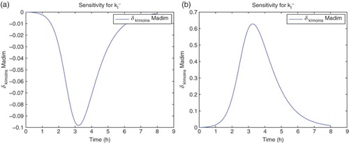
Figure 10. (a) Sensitivity w.r.t. ; (b) sensitivity w.r.t.
.
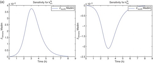
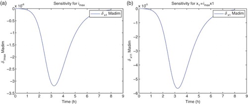
Figure 11. (a) Sensitivity w.r.t. ; (b) sensitivity w.r.t.
.
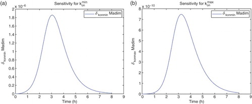
Figure 12. (a) Sensitivity w.r.t. ; (b) sensitivity w.r.t.
.

Figure 13. (a) Sensitivity w.r.t. ; (b) sensitivity w.r.t.
.
Table
Table
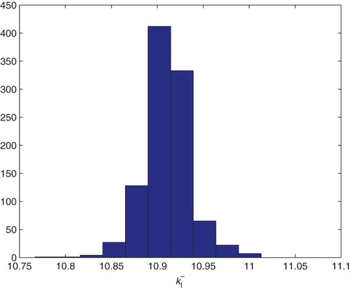
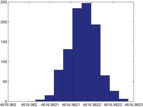
Figure 14. Two parameters estimation (,
). Bootstrapping distribution for
. We use GLS and
runs.
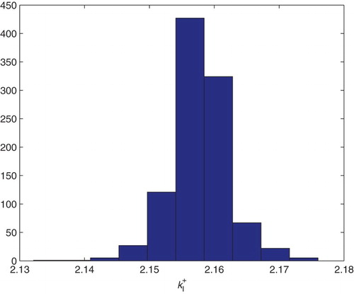
Figure 15. Two parameters estimation (,
). Bootstrapping distribution for
. We use GLS and
runs.
Table
Table
Table
Table
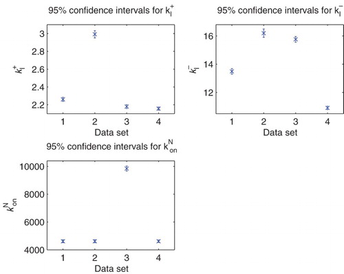
Figure 16. Confidence intervals.
Table
Figure 17. Estimation for ,
and
: bootstrapping distribution for
for GLS and
runs.
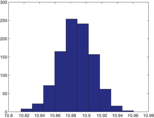
Figure 18. Estimation for ,
, and
: bootstrapping distribution for
for GLS and
runs.
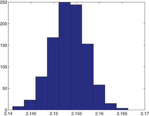
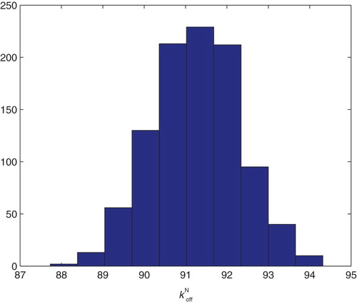
Figure 19. Estimation for ,
, and
: bootstrapping distribution for
for GLS and
runs.
Table
Table
Table
Figure 20. Three parameters estimation (,
and
): bootstrapping distribution for
. We used GLS and
runs.
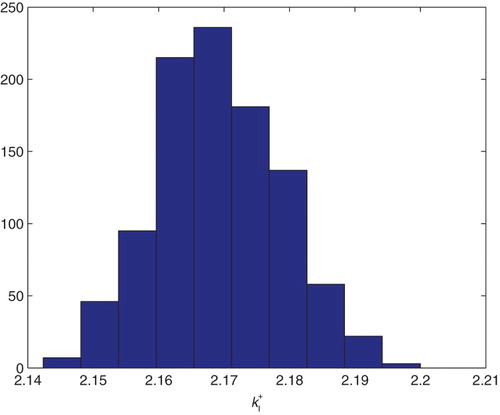
Figure 21. Three parameters estimation (,
and
): bootstrapping distribution for
. We used GLS and
runs.
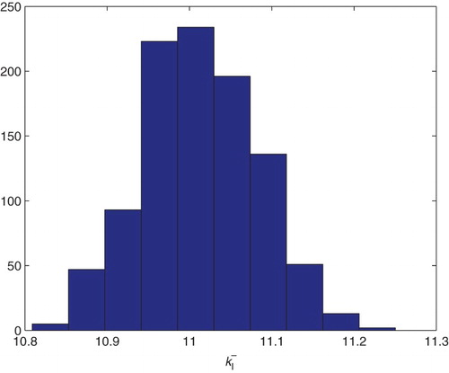
Figure 22. Three parameters estimation (,
and
): bootstrapping distribution for
. We used GLS and
runs.
Table
Table
Table