An optimal control problem for ovine brucellosis with culling

Figures & data

Figure 1. Schematic representation of the model. Note that all rates are dependent on the variable for the group from which they originate (Colour online).

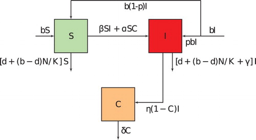
Table 1. Parameter values for ovine brucellosis and their descriptions.

Variable	Description	Dimensions
S:	Number of susceptible subjects
I:	Number of infectious subjects
C:	Proportion of contaminated environment
Parameter	Description	Value per year	Source
b	Per capita birth rate	0.83 births/per subject	[1]
d	Per capita mortality rate	0.79 deaths/subject	[1]
γ	Percentage culling rate	Estimated, $[0,1]$
K	Carrying capacity	1.82 $\times {10}^7$ subjects	[1]
p	Probability of vertical transmission	0.05	[1]
β	Direct transmission	Estimated
α	Indirect transmission	Estimated
η	Contamination rate	Estimated
δ	Disinfection rate	1.82 virus particles	[1]

Table 2. Sensitivity indices of ${\mathcal{R}}_0$ and $i^{\ast }$ to the parameters of the model in Table 1.

	90% culling rate		50% culling rate
Parameter	Sensitivity to ${\mathcal{R}}_0$	Sensitivity to $i^{\ast }$	Sensitivity to ${\mathcal{R}}_0$	Sensitivity to $i^{\ast }$
b	−0.4670	+0.9340	−0.6120	+1.2239
d	–	–	–	–
γ	−0.5330	+1.0660	−0.3880	+0.7761
K	+1.0000	+2.5000	+1.0000	+2.5000
p	+0.0246	−0.0492	+0.0322	−0.0644
β	+1.0000	−2.0000	+1.0000	−2.0000
α	+1.3736e−7	+6.8681e−8	+1.3736e−7	+6.8681e−8
η	+1.3736e−7	−0.5000	+1.3736e−7	−0.5000
δ	−1.3736e−7	+0.5000	−1.3736e−7	+0.5000

Notes: The basic reproduction number at 90% culling rate is 0.6467, for 50% is 0.8475, and a 10% culling rate gives ${\mathcal{R}}_0=\mathrm{1.2290.}$ The indices given in the table arise from 90% and 50%culling rates.

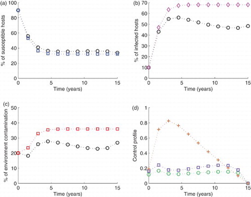
Figure 2. Simulation of the model with $u_1\ne 0,u_2=0,u_3=0.$ The blue circled line in (a), the pink diamond line in (b) and the red squared line in (c) show the model run in the absence of any control effort. In the same figures (i.e. (a), (b) and (c)), the circled black lines represent the variables run in the presence of control efforts described. In subfigure (d), the green circles are for control $u_1,$ purple square for $u_2$, and brown cross are for $u_3$. Other parameter values are given in Table 1 (Colour online).

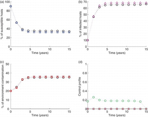
Figure 3. Simulation of the model with $u_1=0,u_2\ne 0,u_3=0.$ The blue circled line in (a), the pink diamond line in (b) and the red squared line in (c) show the model run in the absence of any control effort. In the same figures (i.e. (a), (b) and (c)), the circled black lines represent the variables run in the presence of control efforts described. In subfigure (d), the green circles are for control $u_1$, purple square for $u_2$, and brown cross are for $u_3$. Other parameter values are given in Table 1 (Colour online).

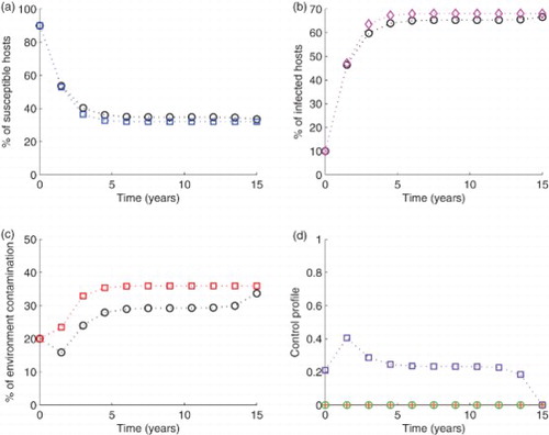
Figure 4. Simulation of the model with $u_1=0,u_2=0,u_3\ne 0.$ The blue circled line in (a), the pink diamond line in (b) and the red squared line in (c) show the model run in the absence of any control effort. In the same figures (i.e. (a), (b) and (c)), the circled black lines represent the variables run in the presence of control efforts described. In subfigure (d), the green circles are for control $u_1$, purple square for $u_2$, and brown cross are for $u_3$. Other parameter values are given in Table 1 (Colour online).

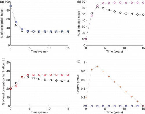
Figure 5. Simulation of the model with $u_1\ne 0,u_2\ne 0,u_3=0.$ The blue circled line in (a), the pink diamond line in (b) and the red squared line in (c) show the model run in the absence of any control effort. In the same figures (i.e. (a), (b) and (c)), the circled black lines represent the variables run in the presence of control efforts described. In subfigure (d), the green circles are for control $u_1$, purple square for $u_2$, and brown cross are for $u_3$. Other parameter values are given in Table 1 (Colour online).

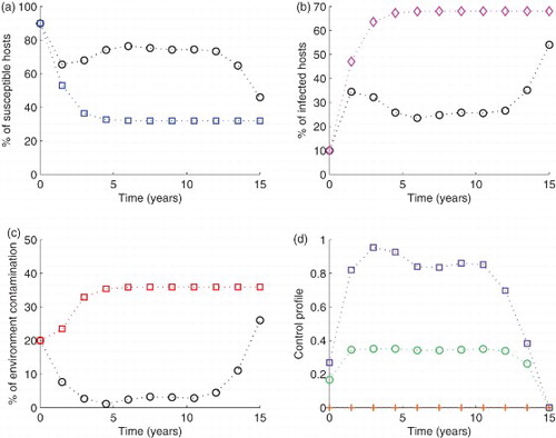
Figure 6. Simulation of the model with $u_1\ne 0,u_2=0,u_3\ne 0.$ The blue circled line in (a), the pink diamond line in (b) and the red squared line in (c) show the model run in the absence of any control effort. In the same figures (i.e. (a), (b) and (c)), the circled black lines represent the variables run in the presence of control efforts described. In subfigure (d), the green circles are for control $u_1$, purple square for $u_2$, and brown cross are for $u_3$. Other parameter values are given in Table 1 (Colour online).

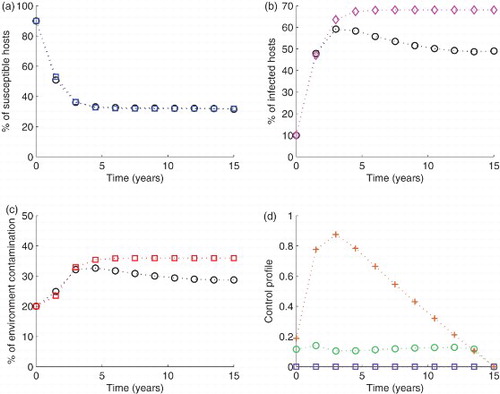
Figure 7. Simulation of the model with $u_1=0,u_2\ne 0,u_3\ne 0.$ The blue circled line in (a), the pink diamond line in (b) and the red squared line in (c) show the model run in the absence of any control effort. In the same figures (i.e. (a), (b) and (c)), the circled black lines represent the variables run in the presence of control efforts described. In subfigure (d), the green circles are for control $u_1$, purple square for $u_2$, and brown cross are for $u_3$. Other parameter values are given in Table 1 (Colour online).

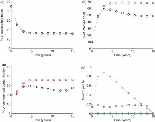
Figure 8. Simulation of the model with $u_1\ne 0,u_2\ne 0,u_3\ne 0.$ The blue circled line in (a), the pink diamond line in (b) and the red squared line in (c) show the model run in the absence of any control effort. In the same figures (i.e. (a), (b) and (c)), the circled black lines represent the variables run in the presence of control efforts described. In subfigure (d), the green circles are for control $u_1$, purple square for $u_2$, and brown cross are for $u_3$. Other parameter values are given in Table 1 (Colour online).

Table 3. Table showing the highest and lowest values (in percentages), for each variable and the times at which they are achieved when different strategies for respective controls are applied.

		$u_1,u_2,u_3=0$	$u_1\ne 0$	$u_2\ne 0$	$u_3\ne 0$	$u_1,u_2\ne 0$	$u_1,u_3\ne 0$	$u_2,u_3\ne 0$	$u_1,u_2,u_3\ne 0$
S	Highest value	90	90	90	90	90	90	90	90
	Time	0	0	0	0	0	0	0	0
	Lowest value	32.08	33.70	33.41	30.22	76.48	31.96	31.96	33.77
	Time	6	15	15	15	6	9	9	15
I	Highest value	68.04	65.30	66.59	61.06	54.10	59.15	58.88	56.19
	Time	9	12	15	3	15	3	3	4.5
	Lowest value	10	10	10	10	10	10	10	10
	Time	0	0	0	0	0	0	0	0
C	Highest value	35.93	35.93	33.71	33.08	26.01	32.62	29.42	27.72
	Time	9	9	15	3	15	3	4.5	4.5
	Lowest value	20	20	15.85	20	2.442	20	20	18.22
	Time	0	0	1.5	0	6	0	0	1.5
$u_1$	At $t=0$	0	0.1683	0	0	0.2	0.1155	0	0.1155
	Highest value	–	0.2595	0	0	0.3442	0.1392	0	0.1660
	Time	0	1.5	–	–	1.5	1.5	–	1.5
$u_2$	At $t=0$	0	0	0.2	0	0.2686	0	0.1395	0.1613
	Highest value	0	0	0.4047	0	0.9542	0	0.1824	0.2419
	Time	–	–	1.5	–	3	–	1.5	1.5
$u_3$	At $t=0$	0	0	0	0.1871	0	0.1878	0.1890	0.1907
	Highest value	0	0	0	0.9060	0	0.8750	0.8823	0.8252
	Time	–	–	–	3	–	3	3	3

B. Aïnseba, C. Benosman, and P. Magal, A model for ovine brucellosis incorporating direct and indirect transmission, J. Biol. Dyn. 4 (2010), pp. 2–11. Available at http://www.math.u-bordeaux1.fr/~pmagal100p/papers/BBM-JBD09.pdf (Accessed 3 July 2012).

 Google Scholar