Figures & data
Figure 1. The menstrual cycle is controlled by hormones secreted by the hypothalamus and the pituitary and by the ovaries. The cycle begins with menstruation and then follicles develop during the follicular phase. Ovulation occurs followed by the luteal phase during which hormones are secreted for pregnancy. The solid arrows indicate the effects of the gonadotropin hormones (red arrows) on the ovaries and the effects of the ovarian hormones (blue arrows) on the brain during the phases of the cycle.
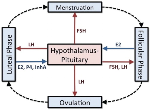
Figure 2. Graphs are taken from Baerwald et al. [Citation3], based on results from Baerwald et al. [Citation1, Citation2]. Panel (a) depicts two follicle waves per cycle and the corpus luteum (yellow body). Panels (b) and (c) graph corresponding LH, FSH, E2, and P4 concentrations. Two-thirds of the women studied had cycles exhibiting two follicle waves per cycle and their results are shown. Note that two follicle waves per cycle corresponds to two rises in FSH. From Baerwald et al. [Citation3] by permission of Oxford University Press. Human Reproduction Update is published on behalf of the European Society of Human Reproduction and Embryology (ESHRE).
![Figure 2. Graphs are taken from Baerwald et al. [Citation3], based on results from Baerwald et al. [Citation1, Citation2]. Panel (a) depicts two follicle waves per cycle and the corpus luteum (yellow body). Panels (b) and (c) graph corresponding LH, FSH, E2, and P4 concentrations. Two-thirds of the women studied had cycles exhibiting two follicle waves per cycle and their results are shown. Note that two follicle waves per cycle corresponds to two rises in FSH. From Baerwald et al. [Citation3] by permission of Oxford University Press. Human Reproduction Update is published on behalf of the European Society of Human Reproduction and Embryology (ESHRE).](/cms/asset/0c5ba22f-5e25-4b96-b39b-ea57950553a3/tjbd_a_1115564_f0002_c.jpg)
Figure 3. Graphs are taken from Baerwald et al. [Citation3], based on results from Baerwald et al. [Citation1, Citation2]. Panel (d) depicts three follicle waves per cycle and the corpus luteum (yellow body). Panels (e) and (f) graph corresponding LH, FSH, E2, and P4 concentrations. One-third of the women studied had cycles exhibiting three follicle waves per cycle and their results are shown. Note that three follicle waves per cycle corresponds to three rises in FSH. From Baerwald et al. [Citation3] by permission of Oxford University Press. Human Reproduction Update is published on behalf of the ESHRE .
![Figure 3. Graphs are taken from Baerwald et al. [Citation3], based on results from Baerwald et al. [Citation1, Citation2]. Panel (d) depicts three follicle waves per cycle and the corpus luteum (yellow body). Panels (e) and (f) graph corresponding LH, FSH, E2, and P4 concentrations. One-third of the women studied had cycles exhibiting three follicle waves per cycle and their results are shown. Note that three follicle waves per cycle corresponds to three rises in FSH. From Baerwald et al. [Citation3] by permission of Oxford University Press. Human Reproduction Update is published on behalf of the ESHRE .](/cms/asset/ba601477-06ee-4840-a82c-265090ed7414/tjbd_a_1115564_f0003_c.jpg)
Figure 4. The brain and the blood compartments for the pituitary model are illustrated. E2, P4, and InhA stimulate (+) and/or inhibit (−) the synthesis and/or release of the pituitary hormones. Clearance from the blood is linear.
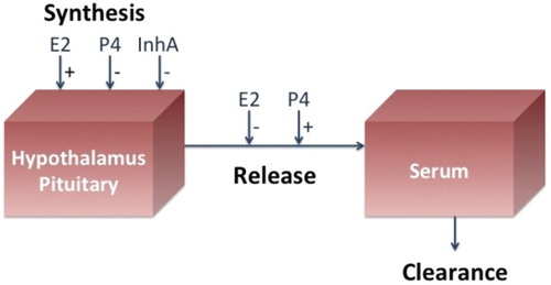
Figure 5. All ovarian follicle stages for the merged model Equations (Equation5(5)
(5) )–(Equation20
(20)
(20) ) with parameters of Table are shown for two cycles. The model maintains two follicle waves for the recruited RcF and growing GrF stages (left panel). The atresia term reduces the dominant stage DomF after mid-cycle and effectively results in small subsequent ovarian stages (right panel).
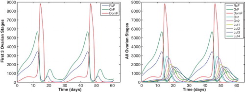
Figure 6. Ovarian hormones E2 and P4 for the merged model Equations (Equation5(5)
(5) )–(Equation20
(20)
(20) ) with parameters of Table are plotted against the McLachlan data [Citation23] for two cycles.
![Figure 6. Ovarian hormones E2 and P4 for the merged model Equations (Equation5(5) ddtRPLH=v0LH+v1LHE2(t−dE)aKmLHa+E2(t−dE)a1+P4(t−dP)KiLH,P−kLH(1+cLH,PP4)RPLH1+cLH,EE2,(5) )–(Equation20(20) InhA=h0+h1DomF+h2Lut2+h3Lut3+h4Lut4.(20) ) with parameters of Table 2 are plotted against the McLachlan data [Citation23] for two cycles.](/cms/asset/d2cfae48-8574-432c-bba9-e146c3fb7213/tjbd_a_1115564_f0006_c.jpg)
Figure 7. Pituitary hormones LH and FSH for the merged model Equations (Equation5(5)
(5) )–(Equation20
(20)
(20) ) with parameters of Table are plotted against the McLachlan data [Citation23] for two cycles.
![Figure 7. Pituitary hormones LH and FSH for the merged model Equations (Equation5(5) ddtRPLH=v0LH+v1LHE2(t−dE)aKmLHa+E2(t−dE)a1+P4(t−dP)KiLH,P−kLH(1+cLH,PP4)RPLH1+cLH,EE2,(5) )–(Equation20(20) InhA=h0+h1DomF+h2Lut2+h3Lut3+h4Lut4.(20) ) with parameters of Table 2 are plotted against the McLachlan data [Citation23] for two cycles.](/cms/asset/2d2017ad-d130-43b2-bd33-6a39c0566e09/tjbd_a_1115564_f0007_c.jpg)
Figure 8. The FSH input function (Equation21(21)
(21) ) has three distinct rises during one cycle and is used to produce three follicle waves.
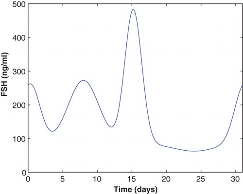
Figure 9. Follicle stages are plotted for Equations (Equation9(9)
(9) )–(Equation20
(20)
(20) ) where the FSH input (Equation21
(21)
(21) ) has three distinct rises. The parameters are given in Table . The left panel depicts the first three stages of follicle growth and isolates waves in the recruited RcF (−) and the growing GrF (−) stages. Note that DomF (−) exhibits only one wave. The right panel gives the complete set of nine follicle stages.
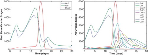
Figure 10. The data of McLachlan et al. [Citation23] for the ovarian hormones are compared to simulations of Equations (Equation9(9)
(9) )–(Equation20
(20)
(20) ) with parameters of Table . The FSH input function (Equation21
(21)
(21) ) with three distinct rises is used.
![Figure 10. The data of McLachlan et al. [Citation23] for the ovarian hormones are compared to simulations of Equations (Equation9(9) ddtRcF=b⋅FSH+c1FSHpKmFp+FSHpRcF−c2LHαRcF,(9) )–(Equation20(20) InhA=h0+h1DomF+h2Lut2+h3Lut3+h4Lut4.(20) ) with parameters of Table 4. The FSH input function (Equation21(21) FSH=82.5+190e−(t−8)210+180e−(t−0.3)20.4+400e−(t−15.2)23−20e−(t−24)215.(21) ) with three distinct rises is used.](/cms/asset/649b7cc7-67ef-46fb-ba7c-ddb3729dbcd3/tjbd_a_1115564_f0010_c.jpg)
Figure 11. The first three stages of ovarian development for the model of follicle wave superfecundation are plotted for two cycles. The parameters are given in Table . The luteal phase DomF (−) stage produces large amounts of luteal E2 which causes a second LH surge, Figure .
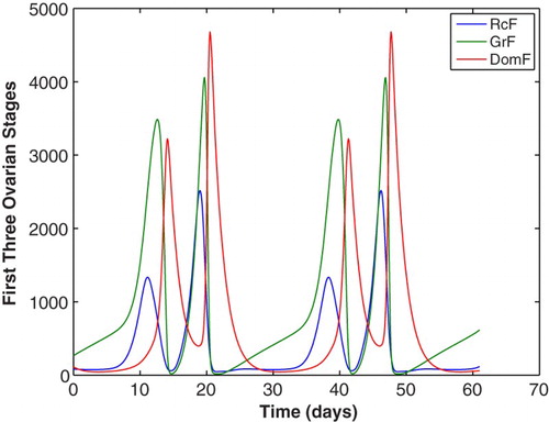
Figure 12. E2 and LH from the model of follicle wave superfecundation is compared to the McLachlan data [Citation28] for two cycles. During one cycle, a second LH surge is present due to increased luteal E2 levels produced by a second dominant follicle. A second LH surge allows for ovulation of the second dominant follicle for potential fertilization resulting in superfecundation.
![Figure 12. E2 and LH from the model of follicle wave superfecundation is compared to the McLachlan data [Citation28] for two cycles. During one cycle, a second LH surge is present due to increased luteal E2 levels produced by a second dominant follicle. A second LH surge allows for ovulation of the second dominant follicle for potential fertilization resulting in superfecundation.](/cms/asset/3779df30-1fbf-4e55-bb94-dbf58f09671a/tjbd_a_1115564_f0012_c.jpg)
Table 1. The five most sensitive parameters ranked in order for model Equations (Equation5 (5) (5) )–(Equation20(20) (20) ) with parameters from Table . The model output for the second column is E2 peak and for the third column is FSH cycle profile. The five most sensitive parameters are the same for both outputs.
Figure 13. This bifurcation diagram plots the maximal LH value along a periodic solution of Equations (Equation5(5)
(5) )–(Equation20
(20)
(20) ) against
with the remaining parameters from Table . SN denotes a saddle-node bifurcation and the * indicates the position of the cycle for best-fit
. The solid blue curve represents stable cycles and the dashed red curve, unstable cycles.
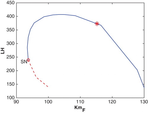
Figure 14. DomF and LH for the superfecundation model for three values of show a diminishing dominant follicle and LH surge during the follicular phase. If
, there is just one ovulation per cycle.
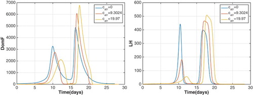
Figure 15. LH profiles for and
illustrating that the period of the stable cycle doubles between these values, that is, a period-doubling bifurcation occurs.
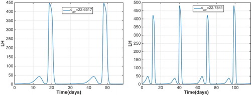
Figure 16. The maximal LH value along a periodic solution of Equations (Equation5(5)
(5) )–(Equation20
(20)
(20) ) is plotted against
with
,
, and the remaining parameters from Table . PD denotes period-doubling bifurcations which occur at
and
. The solid blue curves represent stable cycles and the dashed red curves, unstable cycles.
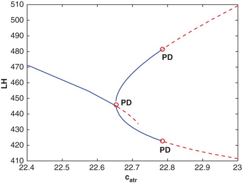
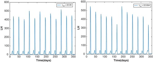
Figure 17. The left panel illustrates the LH profile of a stable, chaotic cycle at . There are 12 LH surges per year but they do not have the same magnitude. The right panel plots the LH profile of a stable cycle of period approximately 180 days at
. This indicates the presence of a period-6 window in the
bifurcation diagram.