A juvenile–adult population model: climate change, cannibalism, reproductive synchrony, and strong Allee effects

Figures & data

Figure 1. A juvenile-adult life cycle graph.

Figure 2. In model (2(2) $\overline{x}(t+1)=P\left(\overline{x}\right(t\left)\right)\overline{x}\left(t\right),$(2) )–(3(3a) $\begin{array}{r}{x}_1(t+1)=b\frac{1}{1+c_2{x}_2\left(t\right)}{x}_2\left(t\right),\end{array}$(3a) ) with parameter values $b=\frac{3}{2}$, $s_1=\frac{1}{2}$, $s_2=\frac{3}{4}$, and $s_3=\frac{1}{2}$, the inherent net reproduction number $R_0=\frac{6}{5}$ is larger than 1. Orbits with initial conditions $(x_1,x_2,x_3)=(10,25,25)$ illustrate the two alternatives in the bifurcating dynamic dichotomy. The coefficient $c_2$ is equal to $\frac{1}{100}$ in both cases. The open squares are the juvenile class densities. The solid (open) circles are the reproductively active (inactive) adult class densities. (a) (Reproductive asynchrony) With $c_g=\frac{1}{100}$ we have $a_{-}=-\frac{7}{3200}<0$. As predicted by Corollary 1 we see that, after some oscillatory transients, the population approaches an equilibrium with both adult classes present at all times. (b) (Reproductive synchrony) With $c_g=1$ we have $a_{-}=\frac{29}{320}>0$. As predicted by Corollary 2 we see that, after some oscillatory transients, the population approaches a synchronous 2-cycle with only one adult class present at all times.

Figure 3. In model (2(2) $\overline{x}(t+1)=P\left(\overline{x}\right(t\left)\right)\overline{x}\left(t\right),$(2) ) with (16(16) $\begin{array}{rl}b& =\beta u\left(\rho \right),s_i={\sigma }_{i}u\left(\rho \right),\\ \beta & >0,0<{\sigma }_i<1,\end{array}$(16) )–(19(19a) $\begin{array}{r}{p}_{23}\left(\overline{x}\right)=\frac{1}{1+c_g{x}_2}{\beta }_3\left(\frac{1}{1+w_1{x}_1}\frac{w_3(1-u(\rho \left)\right)}{1+w_3(1-u(\rho \left)\right)x_3}{x}_1\right),\end{array}$(19a) ) and parameter values $\beta =\frac{33}{20}$, ${\sigma }_1=\frac{11}{20}$, ${\sigma }_2=\frac{33}{40}$ and ${\sigma }_3=\frac{11}{20}$, the inherent net reproduction number $R_0=\frac{6}{5}$ is larger than 1. The coefficient $c_2$ is equal to $\frac{1}{100}$ in both cases. The open squares are the juvenile class densities. The solid (open) circles are the reproductively active (inactive) adult class densities. Initial conditions are $(x_1,x_2,x_3)=(10,25,25)$. (a) (No cannibalism). If cannibalism is absent ($w_2=w_3=0$), we have $a_{-}=-\frac{7}{3200}<0$. As predicted by Corollary 1 we see that, after some oscillatory transients, the population approaches an equilibrium. (b) (Cannibalism) If cannibalism is introduced by setting $w_2=w_3=1$, reproductive synchrony results. Other parameter values are $\rho =10$, $c_{\rho }=1$, $w_1=0.01$, ${\sigma }_{2m}=\frac{38}{40}$, $s_{3m}=\frac{19}{20}$ and $c_{\beta 2}=c_{\beta 3}=1$. the bifurcation diagnostic quantities are $c_w=-0.8936\times {10}^{-3}$ and $c_b=-0.2612\times {10}^{-1}$. Then $a_{+}=-0.3505\times {10}^{-1}<0$ and $a_{-}=0.1718\times {10}^{-1}>0$. As predicted by Corollary 2 we see that, after some oscillatory transients, the population approaches a synchronous 2-cycle.

Figure 4. $\beta =2$, ${\sigma }_1=0.75$, ${\sigma }_2={\sigma }_3=0.50$, $c_{\rho }=20$, $c_2=c_g=0.001$, $w_1=20$, and $w_2=w_3=0$. The open squares are the juvenile class densities. The solid (open) circles are the reproductively active (inactive) adult class densities. Initial conditions are $(x_1,x_2,x_3)=(10,25,25)$. (a) $\rho =90$: In this case $R_0=1.206$ and $c_w=-0.5109\times {10}^{-3}$, $c_b=-0.6068\times {10}^{-4}$, $a_{+}=-0.5716\times {10}^{-4}$, $a_{-}=0.4503\times {10}^{-3}$. (b) $\rho =75$: In this case $R_0=1.107$ and $c_w=-0.4998\times {10}^{-3}$, $c_b=-0.5584\times {10}^{-4}$, $a_{+}=-0.5557\times {10}^{-3}$, $a_{-}=0.4440\times {10}^{-3}$. (c) $\rho =55$: In this case $R_0=0.9320$ and $c_w=-0.4761\times {10}^{-3}$, $c_b=-0.4683\times {10}^{-4}$, $a_{+}=-0.5229\times {10}^{-3}$, $a_{-}=0.4292\times {10}^{-3}$.

Figure 5. The same parameters as in Figure 4 except $c_g=1$. The open squares are the juvenile class densities. The solid (open) circles are the reproductively active (inactive) adult class densities. Initial conditions are $(x_1,x_2,x_3)=(10,25,25)$. (a) $\rho =90$: In this case $R_0=1.206$ and $c_w=-0.5109\times {10}^{-3}$, $c_b=-0.6068\times {10}^{-1}$, $a_{+}=-0.6119\times {10}^{-1}$, $a_{-}=0.6017\times {10}^{-1}$. (b) $\rho =75$: In this case $R_0=1.107$ and $c_w=-0.4998\times {10}^{-3}$, $c_b=-0.5584\times {10}^{-1}$, $a_{+}=-0.5634\times {10}^{-1}$, $a_{-}=0.5534\times {10}^{-1}$. (c) $\rho =55$: In this case $R_0=0.9320$ and $c_w=-0.4761\times {10}^{-3}$, $c_b=-0.4683\times {10}^{-1}$, $a_{+}=-0.4731\times {10}^{-1}$, $a_{-}=0.4636\times {10}^{-1}$.

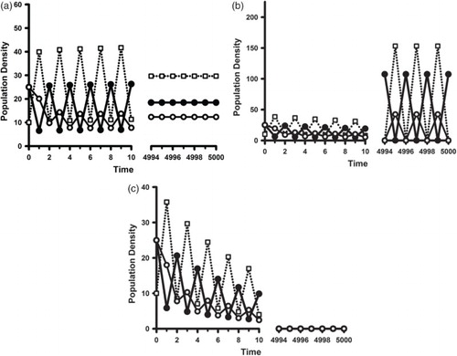
Figure 6. Sample orbits of model (2(2) $\overline{x}(t+1)=P\left(\overline{x}\right(t\left)\right)\overline{x}\left(t\right),$(2) ) with (16(16) $\begin{array}{rl}b& =\beta u\left(\rho \right),s_i={\sigma }_{i}u\left(\rho \right),\\ \beta & >0,0<{\sigma }_i<1,\end{array}$(16) )–(19(19a) $\begin{array}{r}{p}_{23}\left(\overline{x}\right)=\frac{1}{1+c_g{x}_2}{\beta }_3\left(\frac{1}{1+w_1{x}_1}\frac{w_3(1-u(\rho \left)\right)}{1+w_3(1-u(\rho \left)\right)x_3}{x}_1\right),\end{array}$(19a) ) and parameter values $\beta =2$, ${\sigma }_1=0.75$, ${\sigma }_2={\sigma }_3=0.50$, $c_{\rho }=20$, $c_2=0.001$, $c_g=1$, $w_1=20$, $w_2=w_3=5$, ${\sigma }_{2m}={\sigma }_{3m}=0.95$, $c_{\beta 2}=c_{\beta 3}=1$. The open squares are the juvenile class densities. The solid (open) circles are the reproductively active (inactive) adult class densities. Initial conditions are $(x_1,x_2,x_3)=(10,25,25)$. (a) $\rho =90$: In this case $R_0=1.206$ and $c_w=-0.7652\times {10}^{-1}$, $c_b=-0.4112$, $a_{+}=-0.4877$, $a_{-}=0.3346$. (b) $\rho =75$: In this case $R_0=1.107$ and $c_w=-0.8358\times {10}^{-1}$, $c_b=-0.4574$, $a_{+}=-0.5410$, $a_{-}=0.3738$. (c) $\rho =55$: In this case $R_0=0.9320$ and $c_w=-0.9357\times {10}^{-1}$, $c_b=-0.5419$, $a_{+}=-0.6355$, $a_{-}=0.4484$.

Figure 7. Sample orbits of model (2(2) $\overline{x}(t+1)=P\left(\overline{x}\right(t\left)\right)\overline{x}\left(t\right),$(2) ) with (16(16) $\begin{array}{rl}b& =\beta u\left(\rho \right),s_i={\sigma }_{i}u\left(\rho \right),\\ \beta & >0,0<{\sigma }_i<1,\end{array}$(16) )–(19(19a) $\begin{array}{r}{p}_{23}\left(\overline{x}\right)=\frac{1}{1+c_g{x}_2}{\beta }_3\left(\frac{1}{1+w_1{x}_1}\frac{w_3(1-u(\rho \left)\right)}{1+w_3(1-u(\rho \left)\right)x_3}{x}_1\right),\end{array}$(19a) ) and the same parameter values as in Figure 6 except now $c_{\beta 2}=c_{\beta 3}=300$. The open squares are the juvenile class densities. The solid (open) circles are the reproductively active (inactive) adult class densities. Initial conditions are $(x_1,x_2,x_3)=(10,25,25)$. (a) $\rho =90$: In this case $R_0=1.206$ and $c_w=34.01$, $c_b=33.68$, $a_{+}=67.69$, $a_{-}=0.3346$. (b) $\rho =75$: In this case $R_0=1.107$ and $c_w=37.28$, $c_b=36.80$, $a_{+}=73.98$, $a_{-}=0.3738$. (c) $\rho =55$: In this case $R_0=0.9320$ and $c_w=41.66$, $c_b=41.21$, $a_{+}=82.87$, $a_{-}=0.4484$.

Table 1. The direction of bifurcation and the stability properties of the bifurcating continua of positive equilibria and synchronous 2-cycles are determined by the signs of the quantities (10) and (11).

Positive equilibria
	$a_{+}>0$	$a_{+}<0$
Direction of bifurcation	Backward	Forward
Stability property	Unstable	Stable if $a_{-}<0$
		Unstable if $a_{-}>0$
Synchronous 2-cycles
	$c_w>0$	$c_w<0$
Direction of bifurcation	Backward	Forward
Stability property	Unstable	Stable if $a_{-}>0$
		Unstable if $a_{-}<0$