Analysis of HIV models with two time delays

Figures & data

Table 1. Parameters and values used in the models and simulations.

Parameter	Description	Value and unit	References
s	Generation rate of uninfected cells	${10}^4$ cell ml^−1 day^−1	See text
$d_{\mathrm{T}}$	Death rate of uninfected cells	0.01 day^−1	[37]
β	Infection rate	$2.4\times {10}^{-8}$ ml virion^−1 day^−1	[44]
f	Fraction of latency	0.001	[41]
δ	Death rate of infected cells	1 day^−1	[26]
α	Activation rate of latently infected cells	0.01 day^−1	[43]
${\delta }_{\mathrm{L}}$	Death rate of latently infected cells	$4\times {10}^{-3}$ day^−1	See text
${\delta }_1$	Death rate of infected cells that have not started to produce virus	0.05 day^−1	See text
N	Viral burst size	2000 virion cell^−1	[44]
c	Viral clearance rate	23 day^−1	[39]
$d_{\mathrm{E}}$	Death rate of effector cells	0.45 day^−1	[33]
p	Generation rate of effector cells	0.05 day^−1	[33]
$d_x$	Killing rate by effector cells	$3.7\times {10}^{-4}$ ml cell day^−1	[33]

Figure 1. Numerical simulation of model (1(1) $\begin{array}{rl}\frac{\mathrm{d}T}{\mathrm{d}t}& =s-d_{T}T-\beta VT,\\ \frac{\mathrm{d}L}{\mathrm{d}t}& =f\beta V(t-{\tau }_1)T(t-{\tau }_1){\mathrm{e}}^{-{\delta }_1{\tau }_1}-{\delta }_{L}L-\alpha L,\\ \frac{\mathrm{d}I}{\mathrm{d}t}& =(1-f)\beta V(t-{\tau }_2)T(t-{\tau }_2){\mathrm{e}}^{-{\delta }_1{\tau }_2}-\delta I+\alpha L,\\ \frac{\mathrm{d}V}{\mathrm{d}t}& =N\delta I-cV.\end{array}$(1) ) without treatment. The time delay ${\tau }_1$ was fixed to be 0.25 days and ${\tau }_2$ was fixed to be 0.5 days [45]. All the other parameter values are the same as those listed in Table 1.

Figure 2. Numerical simulation of model (1(1) $\begin{array}{rl}\frac{\mathrm{d}T}{\mathrm{d}t}& =s-d_{T}T-\beta VT,\\ \frac{\mathrm{d}L}{\mathrm{d}t}& =f\beta V(t-{\tau }_1)T(t-{\tau }_1){\mathrm{e}}^{-{\delta }_1{\tau }_1}-{\delta }_{L}L-\alpha L,\\ \frac{\mathrm{d}I}{\mathrm{d}t}& =(1-f)\beta V(t-{\tau }_2)T(t-{\tau }_2){\mathrm{e}}^{-{\delta }_1{\tau }_2}-\delta I+\alpha L,\\ \frac{\mathrm{d}V}{\mathrm{d}t}& =N\delta I-cV.\end{array}$(1) ) under treatment. The infection rate β was assumed to be reduced by 90%. The initial conditions were assumed to be the steady states of the model before treatment (see Figure 1). All the other parameter values are the same as those listed in Table 1.

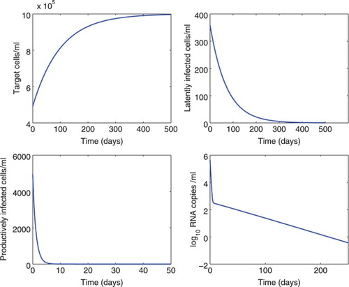
Figure 3. Effect of different time delays (${\tau }_1$) on the dynamics of model (1(1) $\begin{array}{rl}\frac{\mathrm{d}T}{\mathrm{d}t}& =s-d_{T}T-\beta VT,\\ \frac{\mathrm{d}L}{\mathrm{d}t}& =f\beta V(t-{\tau }_1)T(t-{\tau }_1){\mathrm{e}}^{-{\delta }_1{\tau }_1}-{\delta }_{L}L-\alpha L,\\ \frac{\mathrm{d}I}{\mathrm{d}t}& =(1-f)\beta V(t-{\tau }_2)T(t-{\tau }_2){\mathrm{e}}^{-{\delta }_1{\tau }_2}-\delta I+\alpha L,\\ \frac{\mathrm{d}V}{\mathrm{d}t}& =N\delta I-cV.\end{array}$(1) ). The delay ${\tau }_1$ was chosen to be 0.1, 0.2, 0.3, or 0.4 days, and the delay ${\tau }_2$ was fixed at 0.5 days. All the other parameter values are the same as those in Figure 1. The lines of different cases overlap.

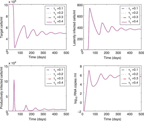
Figure 4. Effect of different time delays (${\tau }_2$) on the dynamics of model (1(1) $\begin{array}{rl}\frac{\mathrm{d}T}{\mathrm{d}t}& =s-d_{T}T-\beta VT,\\ \frac{\mathrm{d}L}{\mathrm{d}t}& =f\beta V(t-{\tau }_1)T(t-{\tau }_1){\mathrm{e}}^{-{\delta }_1{\tau }_1}-{\delta }_{L}L-\alpha L,\\ \frac{\mathrm{d}I}{\mathrm{d}t}& =(1-f)\beta V(t-{\tau }_2)T(t-{\tau }_2){\mathrm{e}}^{-{\delta }_1{\tau }_2}-\delta I+\alpha L,\\ \frac{\mathrm{d}V}{\mathrm{d}t}& =N\delta I-cV.\end{array}$(1) ). The delay ${\tau }_2$ was chosen to be 0.5, 0.6, 0.7, or 0.8 days, and the delay ${\tau }_1$ was fixed at 0.25 days. All the other parameter values are the same as those in Figure 1.

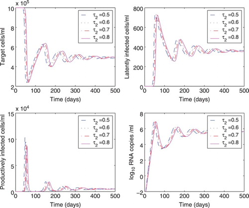
Figure 5. Upper panel: plots of $|a_1\left(j\omega \right)|\pm |a_2\left(j\omega \right)|$ (see Equations (22(22) $a_1\left(\lambda \right)=\frac{-R_{0}c\delta \lambda -d_E{R}_{0}c\delta }{{\lambda }^3+(R_0\delta +d_E+c){\lambda }^2+[d_E{R}_0\delta +c(R_0\delta +d_E\left)\right]\lambda +c{d}_E{R}_0\delta },$(22) ) and (23(23) $a_2\left(\lambda \right)=\frac{(R_0-1)d_E\delta \lambda +c(R_0-1)d_E\delta }{{\lambda }^3+(R_0\delta +d_E+c){\lambda }^2+[d_E{R}_0\delta +c(R_0\delta +d_E\left)\right]\lambda +c{d}_E{R}_0\delta }.$(23) )) as a function of ω. The intersection point of $|a_1\left(j\omega \right)|+|a_2\left(j\omega \right)|$ and 1 is 0.69. Lower panel: stability crossing curves corresponding to the crossing interval (0, 0.69] for the two-delay model (18(18) $\begin{array}{rl}\frac{\mathrm{d}I}{\mathrm{d}t}& =\beta V(t-{\tau }_1)T_0-\delta I-d_{x}EI,\\ \frac{\mathrm{d}V}{\mathrm{d}t}& =N\delta I-cV,\\ \frac{\mathrm{d}E}{\mathrm{d}t}& =pI(t-{\tau }_2)-d_{E}E.\end{array}$(18) ). The basic reproductive number was chosen to be $R_0=2.6$. The other parameters were chosen based on the estimates from data fitting in ref. [33]: $\delta =0.3$ day⁻¹, c=23 day⁻¹, and $d_E=0.45$ day⁻¹.

Figure 6. Upper panel: plots of $|a_1\left(j\omega \right)|\pm |a_2\left(j\omega \right)|$ as a function of ω. The intersection point of $|a_1\left(j\omega \right)|+|a_2\left(j\omega \right)|$ and 1 is 1.12. Lower panel: stability crossing curves corresponding to the crossing interval (0, 1.12] for the two-delay model (18(18) $\begin{array}{rl}\frac{\mathrm{d}I}{\mathrm{d}t}& =\beta V(t-{\tau }_1)T_0-\delta I-d_{x}EI,\\ \frac{\mathrm{d}V}{\mathrm{d}t}& =N\delta I-cV,\\ \frac{\mathrm{d}E}{\mathrm{d}t}& =pI(t-{\tau }_2)-d_{E}E.\end{array}$(18) ). The basic reproductive number was chosen to be $R_0=5$. The other parameters are the same as those in Figure 5.

A.S. Perelson, D.E. Kirschner, and R.J. De Boer, Dynamics of HIV infection of CD4+ T cells, Math. Biosci. 114 (1993), pp. 81–125. doi: 10.1016/0025-5564(93)90043-A

 PubMed Web of Science ®Google Scholar

L. Rong, Z. Feng, and A.S. Perelson, Emergence of HIV-1 drug resistance during antiretroviral treatment, Bull. Math. Biol. 69 (2007), pp. 2027–2060. doi: 10.1007/s11538-007-9203-3

 PubMed Web of Science ®Google Scholar

L. Rong and A.S. Perelson, Modeling Latently infected cell activation: Viral and latent reservoir persistence, and viral blips in HIV-infected patients on potent therapy, PLoS Comput. Biol. 5 (2009), p. e1000533. doi: 10.1371/journal.pcbi.1000533

 PubMed Web of Science ®Google Scholar

M. Markowitz, M. Louie, A. Hurley, E. Sun, M. Di Mascio, A.S. Perelson, and D.D. Ho, A novel antiviral intervention results in more accurate assessment of human immunodeficiency virus type 1 replication dynamics and T-cell decay in vivo, J. Virol. 77 (2003), pp. 5037–5038. doi: 10.1128/JVI.77.8.5037-5038.2003

 PubMed Web of Science ®Google Scholar

L. Rong and A.S. Perelson, Modeling HIV persistence, the latent reservoir, and viral blips, J. Theoret. Biol. 260 (2009), pp. 308–331. doi: 10.1016/j.jtbi.2009.06.011

 PubMed Web of Science ®Google Scholar

B. Ramratnam, S. Bonhoeffer, J. Binley, A. Hurley, L. Zhang, J.E. Mittler, M. Markowitz, J.P. Moore, A.S. Perelson, and D.D. Ho, Rapid production and clearance of HIV-1 and hepatitis C virus assessed by large volume plasma apheresis, Lancet 354 (1999), pp. 1782–1785. doi: 10.1016/S0140-6736(99)02035-8

 PubMed Web of Science ®Google Scholar

K.A. Pawelek, S. Liu, F. Pahlevani, and L. Rong, A model of HIV-1 infection with two time delays: Mathematical analysis and comparison with patient data, Math. Biosci. 235 (2012), pp. 98–109. doi: 10.1016/j.mbs.2011.11.002

 PubMed Web of Science ®Google Scholar

L. Rong, Z. Feng, and A.S. Perelson, Mathematical analysis of age-structured HIV-1 dynamics with combination antiretroviral therapy, SIAM J. Appl. Math. 67 (2007), pp. 731–756. doi: 10.1137/060663945

 Web of Science ®Google Scholar