Modelling and estimation of infectious diseases in a population with heterogeneous dynamic immunity

Figures & data

Figure 1. On the left, we see the function $r\left(\theta \right)$ plotted over the interval $[0,Q]$. Note that the function is not bounded on the whole interval, but is continuous whenever it is bounded. On the right, we show the behaviour of $r\left(\theta \right)$ near its root. We see that it is strictly monotonically increasing there. In particular, $r\left(\theta \right)$ has a unique root given by ${\theta }^{\ast }\approx 0.08707$.

Figure 2. We see for both the susceptible and infected population the theoretical steady states $S_{{\theta }^{\ast }}\left(\omega \right)$ and $I_{{\theta }^{\ast }}\left(\omega \right)$ given by the thick black line. The dashed white lines show $S(300,\omega )$ and $I(300,\omega )$, respectively, where S and I were calculated from system (4(4) $\begin{array}{rl}\frac{\mathrm{\partial }}{\mathrm{\partial }t}S(t,\omega )+\frac{\mathrm{\partial }}{\mathrm{\partial }\omega }\left(d\right(\omega \left)S\right(t,\omega \left)\right)& =-\sigma \left(t\right)p\left(\omega \right){\int }_0^{1}q\left(\zeta \right)I(t,\zeta )\mathrm{d}\zeta S(t,\omega )+\delta \left(\omega \right)I(t,\omega ),\\ \frac{\mathrm{\partial }}{\mathrm{\partial }t}I(t,\omega )+\frac{\mathrm{\partial }}{\mathrm{\partial }\omega }\left(e\right(\omega \left)I\right(t,\omega \left)\right)& =\sigma \left(t\right)p\left(\omega \right){\int }_0^{1}q\left(\zeta \right)I(t,\zeta )\mathrm{d}\zeta S(t,\omega )-\delta \left(\omega \right)I(t,\omega ),\end{array}$(4) ) using an exponential initial condition. We also show the initial conditions and the solution at the earlier point t=20. On the right, we plot $\mathrm{dist}\left(t\right)=\parallel \left(S_{{\theta }^{\ast }}\right(\omega ),I_{{\theta }^{\ast }}(\omega \left)\right)-\left(S\right(t,\omega ),I(t,\omega \left)\right){\parallel }_{L_1}$ to show that the solution does indeed converge towards the steady state.

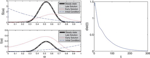
Figure 3. Set-membership estimation of the prevalence $I\left(t\right)$. Note that while for small t the prevalence can take significantly different values for different initial conditions, for large t both the maximum and the minimum converge to the same value. On the right, we show in more detail the interval where the maximum and minimum differ significantly.

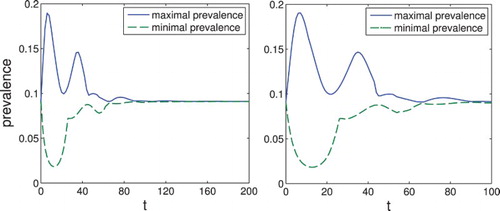
Figure 4. On the left, we show the set-membership estimation of the prevalence for $\sigma =0.25$. It can be seen that the disease dies out. On the right, we show the solution $S(t,\omega )$ with initial condition $u\left(\omega \right)=\phi \left(\omega \right)$. We see that the function does indeed tend towards a Dirac delta at $\omega =0$.

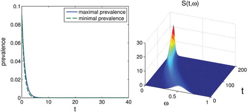
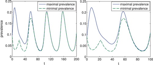
Figure 5. Set-estimation of the prevalence for the system with $\sigma \left(t\right)=2.5(1+\sin (\frac{4\pi }{100}t\left)/100\right)$. The prevalence $I\left(t\right)$ converges to a periodic solution.

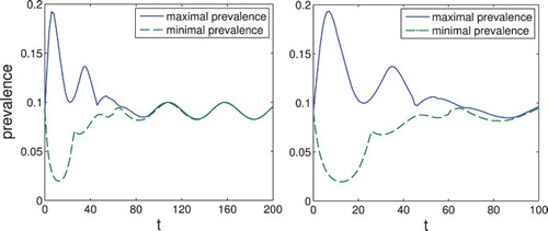
Figure 6. Set-estimation of the prevalence for the system with $\sigma \left(t\right)=2.5(1+\sin (\frac{4\pi }{100}t\left)/10\right)$. The prevalence $I\left(t\right)$ converges again to a periodic solution, but with more pronounced oscillations.