Dual role of delay effects in a tumour–immune system

Figures & data

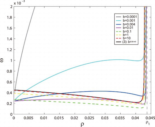
Figure 1. Stability regions of tumour-presence equilibria $E^{\ast }$ and $E^{+}$ and Hopf bifurcation are shown in the $\rho -\omega$ parameter plane.

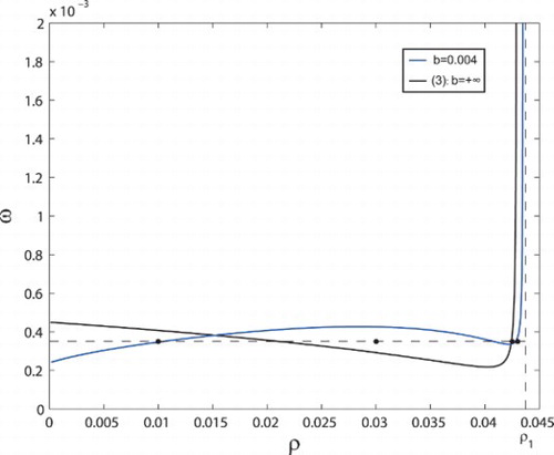
Figure 2. The time evolution curves of system (3(3) $\begin{array}{rl}\frac{\mathrm{d}x\left(t\right)}{\mathrm{d}t}& =\alpha x\left(t\right)(1-\beta x(t\left)\right)-x\left(t\right)y\left(t\right),\\ \frac{\mathrm{d}y\left(t\right)}{\mathrm{d}t}& ={\sigma }_1-{\delta }_{1}y\left(t\right)+\rho y\left(t\right)z\left(t\right),\\ \frac{\mathrm{d}z\left(t\right)}{\mathrm{d}t}& ={\sigma }_2-{\delta }_{2}z\left(t\right)+\omega x\left(t\right)z\left(t\right),\end{array}$(3) ) (left panel) and system (4(4) $\begin{array}{rl}\frac{\mathrm{d}x\left(t\right)}{\mathrm{d}t}& =\alpha x\left(t\right)(1-\beta x(t\left)\right)-x\left(t\right)y\left(t\right),\\ \frac{\mathrm{d}y\left(t\right)}{\mathrm{d}t}& ={\sigma }_1-{\delta }_{1}y\left(t\right)+\rho y\left(t\right)G\left(t\right),\\ \frac{\mathrm{d}z\left(t\right)}{\mathrm{d}t}& ={\sigma }_2-{\delta }_{2}z\left(t\right)+\omega x\left(t\right)z\left(t\right),\\ \frac{\mathrm{d}G\left(t\right)}{\mathrm{d}t}& =bz\left(t\right)-bG\left(t\right),\end{array}$(4) ) (right panel). Here, we fix $\omega =0.00035$, b=0.004 and choose four different ρ as 0.01 (a and b), 0.03 (c and d), 0.0425 (e and f), 0.043 (g and h). (a) Local asymptotic stability of ${\tilde{E}}_1^{\ast }$. (b) The time evolution curves of system (4(4) $\begin{array}{rl}\frac{\mathrm{d}x\left(t\right)}{\mathrm{d}t}& =\alpha x\left(t\right)(1-\beta x(t\left)\right)-x\left(t\right)y\left(t\right),\\ \frac{\mathrm{d}y\left(t\right)}{\mathrm{d}t}& ={\sigma }_1-{\delta }_{1}y\left(t\right)+\rho y\left(t\right)G\left(t\right),\\ \frac{\mathrm{d}z\left(t\right)}{\mathrm{d}t}& ={\sigma }_2-{\delta }_{2}z\left(t\right)+\omega x\left(t\right)z\left(t\right),\\ \frac{\mathrm{d}G\left(t\right)}{\mathrm{d}t}& =bz\left(t\right)-bG\left(t\right),\end{array}$(4) ) around ${\tilde{E}}_1^{+}$ show periodic oscillations. (c) The time evolution curves of system (3(3) $\begin{array}{rl}\frac{\mathrm{d}x\left(t\right)}{\mathrm{d}t}& =\alpha x\left(t\right)(1-\beta x(t\left)\right)-x\left(t\right)y\left(t\right),\\ \frac{\mathrm{d}y\left(t\right)}{\mathrm{d}t}& ={\sigma }_1-{\delta }_{1}y\left(t\right)+\rho y\left(t\right)z\left(t\right),\\ \frac{\mathrm{d}z\left(t\right)}{\mathrm{d}t}& ={\sigma }_2-{\delta }_{2}z\left(t\right)+\omega x\left(t\right)z\left(t\right),\end{array}$(3) ) around ${\tilde{E}}_2^{\ast }$ show periodic oscillations. (d) Local asymptotic stability of ${\tilde{E}}_2^{+}$. (e) Local asymptotic stability of ${\tilde{E}}_3^{\ast }$. (f) The time evolution curves of system (4(4) $\begin{array}{rl}\frac{\mathrm{d}x\left(t\right)}{\mathrm{d}t}& =\alpha x\left(t\right)(1-\beta x(t\left)\right)-x\left(t\right)y\left(t\right),\\ \frac{\mathrm{d}y\left(t\right)}{\mathrm{d}t}& ={\sigma }_1-{\delta }_{1}y\left(t\right)+\rho y\left(t\right)G\left(t\right),\\ \frac{\mathrm{d}z\left(t\right)}{\mathrm{d}t}& ={\sigma }_2-{\delta }_{2}z\left(t\right)+\omega x\left(t\right)z\left(t\right),\\ \frac{\mathrm{d}G\left(t\right)}{\mathrm{d}t}& =bz\left(t\right)-bG\left(t\right),\end{array}$(4) ) around ${\tilde{E}}_3^{+}$ show periodic oscillations. (g ) Local asymptotic stability of ${\tilde{E}}_4^{\ast }$. (h) Local asymptotic stability of ${\tilde{E}}_4^{+}$.

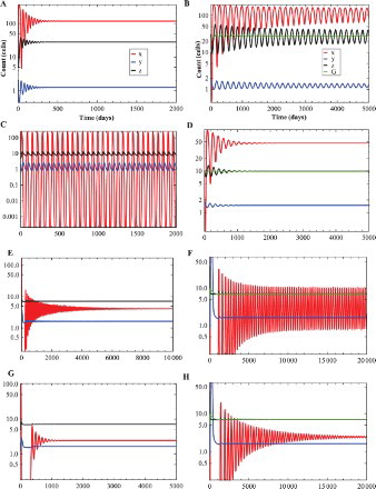
Figure 3. The curves of $Q\left(b\right)$ with respect to b. Case (I): we choose $(\rho ,\omega )=(0.0436,0.00035)$, and we have $Q\left(b\right)>0$ when b>0. Case (II): we choose $(\rho ,\omega )=(0.043,0.0001)$, and we have $Q\left(b\right)>0$ when b>0. Case (III): we choose $(\rho ,\omega )=(0.043,0.00035)$, and we have $Q\left(b\right)>0$ when $0<b<\underset{\_}{b}=0.00433351$ or $b>\overline{b}=0.219156$.

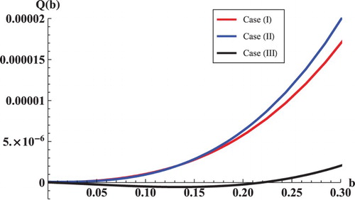
Figure 4. Hopf bifurcation curves of $E^{+}$ are shown in the $\rho -\omega$ parameter plane for a different b.