An age-structured within-host HIV-1 infection model with virus-to-cell and cell-to-cell transmissions

Figures & data

Table 1. The definitions of the parameters in system (4(4) $\begin{array}{rl}& \dot{x}\left(t\right)=s-\mathrm{d}x\left(t\right)-\frac{\beta x\left(t\right)v\left(t\right)}{1+\alpha v\left(t\right)}-x\left(t\right){\int }_0^{\mathrm{\infty }}{\beta }_1\left(a\right)y(a,t)\mathrm{d}a,\\ & \frac{\mathrm{\partial }y(a,t)}{\mathrm{\partial }t}+\frac{\mathrm{\partial }y(a,t)}{\mathrm{\partial }a}=-\mu \left(a\right)y(a,t),\\ & \dot{v}\left(t\right)={\int }_0^{\mathrm{\infty }}k\left(a\right)y(a,t)\mathrm{d}a-uv\left(t\right),\end{array}$(4) ).

Parameters	Description
s	The recruitment rate of healthy T cells
d	The per capita death rate of uninfected cells
u	Clearance rate of virions
α	Saturation constant
β	The rate at which an uninfected cell becomes infected by an infectious virus
a	Age of infection, that is, the time since an HIV virion penetrated cell
${\beta }_1\left(a\right)$	The infection rate of productively infected cells with age a
$\mu \left(a\right)$	The age-dependent per capita death rate of infected cells
$k\left(a\right)$	The viral production rate of an infected cell with age a

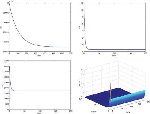
Figure 1. The temporal solution found by numerical integration of system (4(4) $\begin{array}{rl}& \dot{x}\left(t\right)=s-\mathrm{d}x\left(t\right)-\frac{\beta x\left(t\right)v\left(t\right)}{1+\alpha v\left(t\right)}-x\left(t\right){\int }_0^{\mathrm{\infty }}{\beta }_1\left(a\right)y(a,t)\mathrm{d}a,\\ & \frac{\mathrm{\partial }y(a,t)}{\mathrm{\partial }t}+\frac{\mathrm{\partial }y(a,t)}{\mathrm{\partial }a}=-\mu \left(a\right)y(a,t),\\ & \dot{v}\left(t\right)={\int }_0^{\mathrm{\infty }}k\left(a\right)y(a,t)\mathrm{d}a-uv\left(t\right),\end{array}$(4) ) with the boundary condition (5(5) $y(0,t)=\frac{\beta x\left(t\right)v\left(t\right)}{1+\alpha v\left(t\right)}+x\left(t\right){\int }_0^{\mathrm{\infty }}{\beta }_1\left(a\right)y(a,t)\mathrm{d}a,t>0,$(5) ) and the initial condition $x\left(0\right)={10}^6$ ml⁻¹, $v\left(0\right)={10}^{-6}$ ml⁻¹, and the parameters $\beta =2.4\times {10}^{-8}$ ml day⁻¹, ${\beta }_1\left(a\right)={10}^{-6}$ ml day⁻¹.

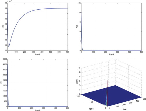
Figure 2. The temporal solution found by numerical integration of system (1.4) with the boundary condition (1.5) and initial condition $x\left(0\right)={10}^6$ ml⁻¹, $v\left(0\right)={10}^{-6}$ ml⁻¹, and the parameters $\beta =2.4\times {10}^{-8}$ ml day⁻¹, ${\beta }_1\left(a\right)=0$ ml day⁻¹.

Figure 3. The temporal solution found by numerical integration of system (4(4) $\begin{array}{rl}& \dot{x}\left(t\right)=s-\mathrm{d}x\left(t\right)-\frac{\beta x\left(t\right)v\left(t\right)}{1+\alpha v\left(t\right)}-x\left(t\right){\int }_0^{\mathrm{\infty }}{\beta }_1\left(a\right)y(a,t)\mathrm{d}a,\\ & \frac{\mathrm{\partial }y(a,t)}{\mathrm{\partial }t}+\frac{\mathrm{\partial }y(a,t)}{\mathrm{\partial }a}=-\mu \left(a\right)y(a,t),\\ & \dot{v}\left(t\right)={\int }_0^{\mathrm{\infty }}k\left(a\right)y(a,t)\mathrm{d}a-uv\left(t\right),\end{array}$(4) ) with the boundary condition (5(5) $y(0,t)=\frac{\beta x\left(t\right)v\left(t\right)}{1+\alpha v\left(t\right)}+x\left(t\right){\int }_0^{\mathrm{\infty }}{\beta }_1\left(a\right)y(a,t)\mathrm{d}a,t>0,$(5) ) and the initial condition $x\left(0\right)={10}^6$ ml⁻¹, $v\left(0\right)={10}^{-6}$ ml⁻¹, and the parameters $\beta =2.4\times {10}^{-10}$ ml day⁻¹, ${\beta }_1\left(a\right)=9\times {10}^{-9}$ ml day⁻¹.