Homogenization techniques for population dynamics in strongly heterogeneous landscapes

Figures & data

Figure 1. Comparison of the travelling wave solution ρ with the leading order approximation ${\rho }_0$ at time t=10 in the logistic growth example. The inset graph shows a ‘zoomed-in’ plot of the leading order approximation ${\rho }_0$ (red dashed) and the numerical non-homogenized solution ρ (black). The main graph shows the numerical non-homogenized solution (black curve) and the upper and lower bound obtained from the homogenized solution. The top red curve is the upper bound g while the bottom red curve is the lower bound g/k. The parameters are $D_1=D_2=1$, $l_1=l_2=0.1$, ${\lambda }_i={\mu }_i=1$, and $\alpha =0.75$ (k=3).

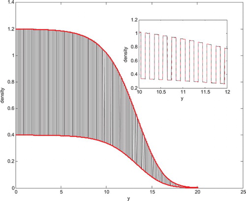
Figure 2. The effect of varying $l_2$ on the accuracy of the leading order approximation of the travelling wave profile. In plots (a–d) $l_2=1.9$ and the numerical non-homogenized solution ρ (black) and leading order approximation ${\rho }_0$ (red) are plotted as a function of the scaled spatial variable ξ (left column) and the unscaled spatial variable x (right column). The first row corresponds to the case where $\alpha =0.25$ andthere is greater preference for patch 2. The second row corresponds to the case where $\alpha =0.75$ and there is greater preference for patch 1. Finally, plot (e) shows the maximum absolute error ($\underset{\xi }{max}|\rho -{\rho }_0|$) as $l_2$ is varied. Plot (f) shows the averaged absolute error across rescaled space ξ. In all cases we ignore population dynamics with $f_1=f_2=0$ and $D_1=D_2=1$ and $l_1=0.1$. We use a Gaussian initial condition and compare solutions at t=3.

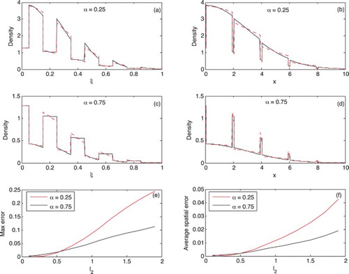
Figure 3. Asymptotic wave speed plotted as a function of patch preference, α. The solid line illustrates the homogenized wave speed prediction (Equation 79(79) $c^{\ast }=2\left(\frac{l_1+l_2}{l_1+l_2/k}\right)\sqrt{\frac{{\lambda }_1{l}_1+{\lambda }_2{l}_2/k}{l_1/D_1+\left(l_2/k\right)/\left(D_2/k^2\right)}}.$(79) ) in the case ${\lambda }_1={\lambda }_2=1$, and the dashed line illustrates the case ${\lambda }_1=1$, ${\lambda }_2=0.5$. The grey stars are the numerically simulated wave speeds obtained from solving the original non-homogenized Equations (2(2) ${\mathrm{\partial }}_{\tau }\rho =D_i{\mathrm{\partial }}_y^2\rho +{\epsilon }^2{f}_i\left(\rho \right)\mathrm{for}y\in (y_{i-1},y_i),i\in \mathbb{Z}.$(2) ), (3(3) $D_{i+1}{\mathrm{\partial }}_y\rho (y_i^{+},\tau )=D_i{\mathrm{\partial }}_y\rho (y_i^{-},\tau ).$(3) ), (7(7) $\rho (y_i^{+},\tau )=k_i\rho (y_i^{-},\tau ).$(7) ). The solution was solved until t=50, and the last 30 time steps were used to estimate wave speed, taking a threshold of 0.01 to track the location of the wave front at each time point. In all cases the population dynamics are given by logistic growth ($f_i\left(\rho \right)=({\lambda }_i-{\mu }_i\rho )\rho$), and parameters are $D_1=D_2=1$, ${\mu }_i=1$ and $l_1=l_2=1$.