Equilibrium Distributions of Populations of Biological Species on Networks of Social Sites

Figures & data

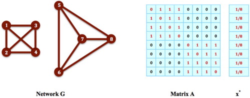
Figure 1. Social Networking Game: Given a network of social sites G and its adjacency matrix A as shown in the figure, $x^{\ast }=(1/4,1/4,1/4,1/4,0,0,0,0{)}^T$ is an equilibrium state of the social networking game on G, meaning that $x^{\ast }$ is an equilibrium distribution of the population on G and also an equilibrium strategy for every individual species such that the social contact of each species achieves its maximum $x^{\ast T}A{x}^{\ast }=3/4$.

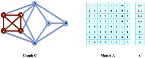
Figure 2. Solitary Inhabiting Game: Given a network of social sites G and its adjacency matrix B with its diagonal elements all set to 1 as shown in the figure, the solitary inhabiting game on G is equivalent to the social networking game on the network complementary to G, which is the same network in Figure 1. Therefore, the equilibrium state of the social networking game in Figure 1, $x^{\ast }=(1/4,1/4,1/4,1/4,0,0,0,0{)}^T$, is also an equilibrium state of the solitary inhabiting game on G in the above figure, meaning that $x^{\ast }$ is an equilibrium distribution of the population on G and also an equilibrium strategy for every individual species in the population such that the social contact of each species achieves its minimum $x^{\ast T}B{x}^{\ast }=1/4$.

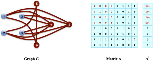
Figure 3. Populations on Cliques: In network G, the nodes $\{1,2,3\}$ form a network clique. Let $x^{\ast }$ be a strategy for choosing this clique, $x_1^{\ast }=x_2^{\ast }=x_3^{\ast }=1/3$ and $x_i^{\ast }=0$ for all $i=4,\dots ,8$. Then, $x^{\ast T}A{x}^{\ast }=(A{x}^{\ast }{)}_i=2/3$ for all i such that $x_i^{\ast }>0$, i.e. $i=1,2,3$. However, $x^{\ast T}A{x}^{\ast }\ge (A{x}^{\ast }{)}_i$ does not hold for all i such that $x_i^{\ast }=0$, i.e. $i=4,\dots ,8$, since $x^{\ast T}A{x}^{\ast }=2/3<(A{x}^{\ast }{)}_4=1$. By Theorem 2.1, $x^{\ast }$ cannot be an equilibrium strategy for the game on G.

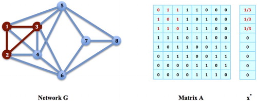
Figure 4. Populations on Maximal Cliques: The nodes $\{1,2,3,4\}$ in G form a maximal clique. Let $x^{\ast }$ be a strategy on this clique, $x_1^{\ast }=x_2^{\ast }=x_3^{\ast }=x_4^{\ast }=1/4$ and $x_i^{\ast }=0$ for all $i=5,\dots ,8$. Then, $x^{\ast T}A{x}^{\ast }=(A{x}^{\ast }{)}_i=3/4$ for all i such that $x_i^{\ast }>0$, i.e. $i=1,2,3,4$, and also, $x^{\ast T}A{x}^{\ast }\ge (A{x}^{\ast }{)}_i$ for all i such that $x_i^{\ast }=0$, i.e. $i=5,\dots ,8$. Then, $x^{\ast }$ satisfies all the conditions in Theorem 2.1, and must be an equilibrium strategy for the social networking game on G.

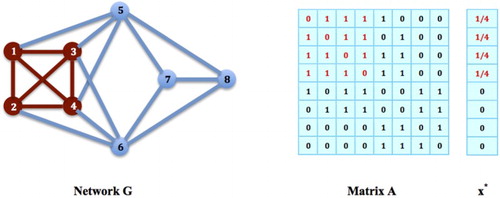
Figure 5. Non-Clique Strategies: The nodes $\{1,2,3,4,5\}$ in G do not form a network clique, but the strategy $x^{\ast }$, $x_1^{\ast }=x_3^{\ast }=x_4^{\ast }=1/4$, $x_2^{\ast }=x_5^{\ast }=1/8$, and $x_i^{\ast }=0$ for $i=6,7,8$, is in fact an equilibrium strategy: It is easy to verify that $x^{\ast T}A{x}^{\ast }=(A{x}^{\ast }{)}_i=3/4$ for all i such that $x_i^{\ast }>0$, i.e. i=1,2,3,4,5, and also, $x^{\ast T}A{x}^{\ast }\ge (A{x}^{\ast }{)}_i$ for all i such that $x_i^{\ast }=0$, i.e. i=6,7,8. Then, $x^{\ast }$ satisfies all the conditions in Theorem 2.1, and must be an equilibrium strategy for the social networking game on G.

Figure 6. Populations on Maximal Cliques vs. Local Contact Maximizers: The nodes $\{1,2,3,4\}$ in G form a maximal network clique. It is an equilibrium strategy for the social networking game on G, but not a local maximizer of the corresponding contact maximization problem: Let $x^{\ast }$ be the equilibrium distribution on this clique, $x_i^{\ast }=1/4$ for all $i=1,\dots ,4$ and $x_i^{\ast }=0$ for all $i=5,\dots ,8$. Construct a new distribution $x=x^{\ast }+p$, where $p=(-2ϵ,0,0,0,ϵ,ϵ,0,0{)}^T$ for a small $ϵ>0$. Then, it is easy to verify that $x_i\ge 0$ for all $i=1,\dots ,8$, $\sum _i{x}_i=1$, and $x^{T}Ax=x^{\ast T}A{x}^{\ast }+2{ϵ}^2>x^{\ast T}A{x}^{\ast }$ for all small $ϵ>0$. As ε goes to zero, x is arbitrarily close to $x^{\ast }$, yet $x^{T}Ax>x^{\ast }A{x}^{\ast }$. Therefore, $x^{\ast }$ cannot be a local maximizer for the corresponding contact maximization problem.

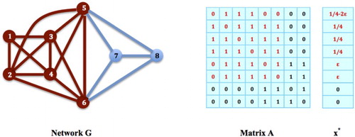
Figure 7. Strict Local Maximizer: The nodes $\{1,2,3,4\}$ in G form a maximal clique. The strategy $x^{\ast }$ on this clique for the social networking game on G, $x_i^{\ast }=1/4$ for all $i=1,\dots ,4$ and $x_i^{\ast }=0$ for all $i=5,\dots ,8$, is a local maximizer of the corresponding contact maximization problem, and $x^{\ast T}A{x}^{\ast }\ge x^{T}Ax$ for any $x\in S$ in a small neighbourhood U of $x^{\ast }$. However, if we choose $x\ne x^{\ast }$ such that $x_1=x_3=x_4=1/4$, $x_2=1/4-ϵ$, $x_5=ϵ$, and $x_i=0$ for i=6,7,8, we see for any U that $x\in S\cap U$ for sufficiently small $ϵ>0$, and $x^{T}Ax=x^{\ast T}A{x}^{\ast }=3/4$. Therefore, $x^{\ast }$ is not a strict local maximizer for the contact maximization problem.

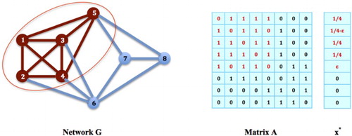
Figure 8. Recovering Maximum Clique Strategies: In the network on the top, the nodes $\{1,2,3,4,5,6\}$ form a subnetwork H, and $x^{\ast }\in S$, $x_i^{\ast }>0$ for all $i\in V_H$ and $x_i^{\ast }=0$ for all $i\in V\mathrm{\setminus }{V}_H$, is a global maximizer for the contact maximization problem. However, H is not a maximum clique. Since node 2 and 6 are not connected, we therefore add 1/8 to $x_2$ but subtract it from $x_6$. We then obtain a reduced subnetwork H, with $V_H=\{1,2,3,4,5\}$, $E_H=\left\{\right(i,j)\in E:i,j\in V_H\}$, as shown in the second network to the top. The solution $x^{\ast }\in S$, $x_i^{\ast }>0$ for all $i\in V_H$ and $x_i^{\ast }=0$ for all $i\in V\mathrm{\setminus }{V}_H$, remains to be a global maximizer for the contact maximization problem. Next, since node 1 and 5 are still not connected, we then add 1/8 to $x_1$ but subtract it from $x_5$ to obtain a further reduced subnetwork$H=(V_H,E_H)$, $V_H=\{1,2,3,4\}$, $E_H=\left\{\right(i,j):i,j\in V_H\}$, as shown in the network in the bottom. The solution $x^{\ast }\in S$, $x_i^{\ast }>0$ for all $i\in V_H$ and $x_i^{\ast }=0$ for all $i\in V\mathrm{\setminus }{V}_H$, again remains to be a global maximizer for the contact maximization problem, but this time, H is a maximum clique of G.

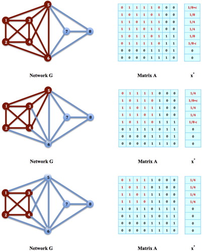
Figure 9. Equilibrium Distributions on Non-clique Subnetworks: One of the equilibrium strategies of the social networking game on network G is when the population is distributed on the two disconnected network cliques, with $x_i^{\ast }=1/8$ for all $i=1,\dots ,8$. It is easy to verify that this strategy is not a local maximizer of the corresponding contact maximization problem and thereby, is not even weakly evolutionarily stable.