Figures & data
Figure 1. Period-doubling bifurcations in the disease-free Equation (Equation15(15)
(15) ), where d=0.5, b=0.1, on the horizontal axis
and on the vertical axis
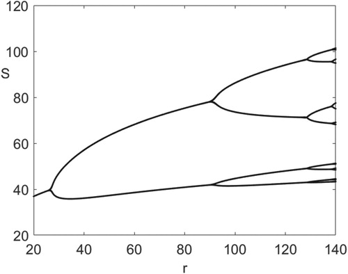
Figure 2. Bifurcation diagram for SIR model: As increases from values less than 1 to values greater than 1, the model dynamics changes from disease extinction to disease persistence on a locally asymptotically stable period 2 population cycle.
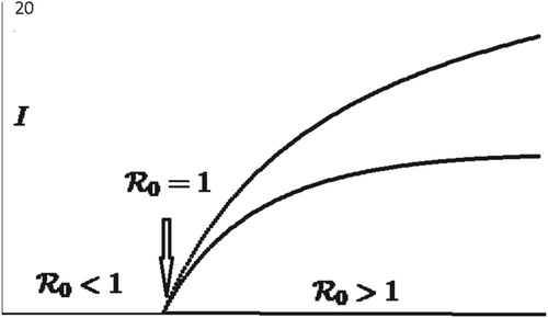
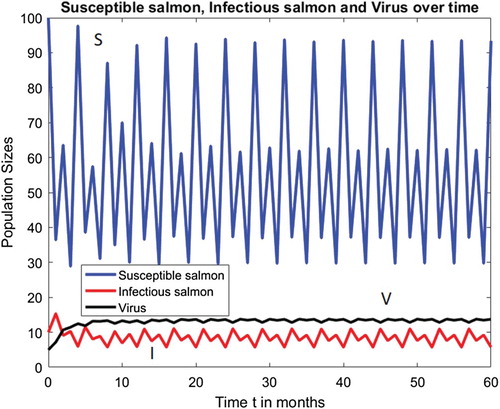
Figure 3. Model (Equation7(7)
(7) ) with
has a locally asymptotically stable endemic period-2 population cycle when
.
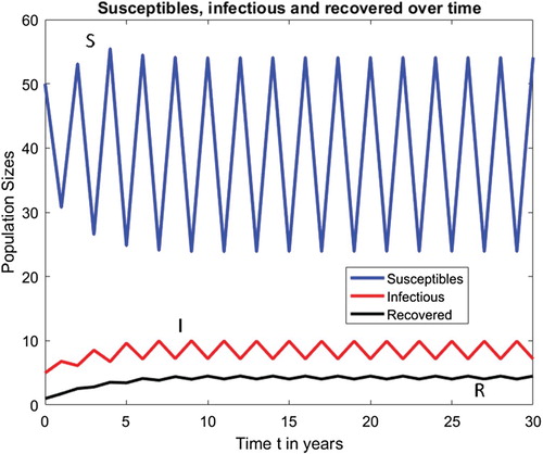
Figure 4. Susceptible and recovered disease-free populations of Model (Equation19(19)
(19) ) undergo period-doubling bifurcations as r is varied between 20 and 140, where p=0.78, d=0.5 and b=0.1.
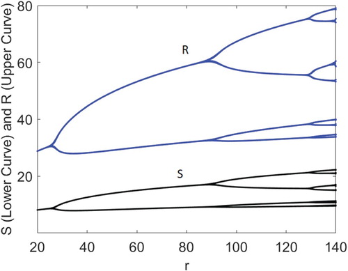
Figure 5. Bifurcation diagram for ISAv Model (Equation20(20)
(20) ): As
increases from values less than 1 to values greater than 1, the model dynamics changes from disease extinction to disease persistence on a periodic or chaotic population cycle.
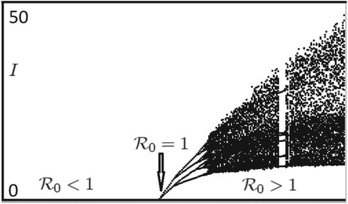
Figure 6. Model (Equation20(20)
(20) ) with
has a locally asymptotically stable period 4 population cycle when
and all the other parameter values are kept fixed at their current values in Figure .