Combination of singularly perturbed vector field method and method of directly defining the inverse mapping applied to complex ODE system prostate cancer model

Figures & data

Table 1. Parameters used in the model (4(4) $\begin{array}{rl}\frac{\mathrm{d}{N}_1}{\mathrm{d}t}& =\underset{\mathrm{proliferation}\mathrm{and}\mathrm{death}}{\underbrace{\left({\alpha }_1\frac{A}{A+k_1}-{\beta }_1\left(k_2+(1-k_2)\frac{A}{A+k_3}\right)\right)N_1}}\\ & -\underset{\mathrm{mutation}\mathrm{to}\mathrm{AI}}{\underbrace{m_1\left(1-\frac{A}{a_0}\right)N_1}}-\underset{\mathrm{killed}\mathrm{by}\mathrm{T}\mathrm{cells}}{\underbrace{-\frac{e_1{N}_{1}T}{g_1+N_1}}}\equiv F_1\left(\overrightarrow{V}\right),\end{array}$(4) )–(9(9) $\frac{\mathrm{d}D}{\mathrm{d}t}=\underset{\mathrm{natural}\mathrm{death}}{\underbrace{-cD}}\equiv F_6\left(\overrightarrow{V}\right),$(9) ).

Parameter	Value	Description
${\alpha }_1$	0.025	AD cell proliferation rate
${\alpha }_2$	0.006/day	AI cell net growth rate
${\beta }_1$	0.008/day	AD cell death rate
$k_1$	2 ng/mL	AD cell proliferation rate dependence on androgen
$k_2$	8	Effect of low androgen level on AD cell death rate
$k_3$	0.5 ng/mL	AD cell death rate dependence on androgen
$e{m}_{4}1$	0.00005/day	maximum mutation rate
$a_0$	30 ng/mL	Normal androgen concentration
γ	0.08/day	Androgen clearance and production rate
ω	10/day	Cytokine clearance rate
μ	0.03/day	T cell death rate
c	0.14/day	Dendritic cell death rate

Table 2. Parameters used in the model (4(4) $\begin{array}{rl}\frac{\mathrm{d}{N}_1}{\mathrm{d}t}& =\underset{\mathrm{proliferation}\mathrm{and}\mathrm{death}}{\underbrace{\left({\alpha }_1\frac{A}{A+k_1}-{\beta }_1\left(k_2+(1-k_2)\frac{A}{A+k_3}\right)\right)N_1}}\\ & -\underset{\mathrm{mutation}\mathrm{to}\mathrm{AI}}{\underbrace{m_1\left(1-\frac{A}{a_0}\right)N_1}}-\underset{\mathrm{killed}\mathrm{by}\mathrm{T}\mathrm{cells}}{\underbrace{-\frac{e_1{N}_{1}T}{g_1+N_1}}}\equiv F_1\left(\overrightarrow{V}\right),\end{array}$(4) )–(9(9) $\frac{\mathrm{d}D}{\mathrm{d}t}=\underset{\mathrm{natural}\mathrm{death}}{\underbrace{-cD}}\equiv F_6\left(\overrightarrow{V}\right),$(9) ).

Parameter	Value	Description
$e_1$	0–1/day	Max rate T cells kill AD cancer cells
$e_2$	$20\cdot {10}^6$cells/day	Max rate T cells kill AI cancer cells
$e_3$	0.1245/day	Maximum rate of clonal expansion
$e_4$	$5\cdot {10}^{-6}$ ng/mL/cell/day	Maximum rate T cells produce IL-2
$g_1$	$10\cdot {10}^9$ cells	Cancer cell saturation level for T-cell kill rate
$g_2$	$400\cdot {10}^6$cells	DC saturation level for T-cell activation
$g_3$	1000 ng/mL	IL-2 saturation level for T-cell clonal expansion
$g_4$	$10\cdot {10}^9$ cells	Cancer cell saturation level for T-cell stimulation
$c_1$	$1\cdot {10}^{-9}$ ng/mL/cell	AD cell PSA-level correlation
$c_2$	$1\cdot {10}^{-9}$ ng/mL/cell	AI cell PSA-level correlation

Note: The biological meaning of $e_1=e_2$ is that T cells are able to kill AD and AI cancer cells equivalently.

Figure 1. The solution profiles of $N_1\left(t\right)$, the androgen-dependent cancer cells. 1: MDDIM, 2: QSS, Quasi-steady state approximation, 3: numerical simulations for the full model. These cancer cells grow at the beginning of the treatment, then after they decrease very quickly.

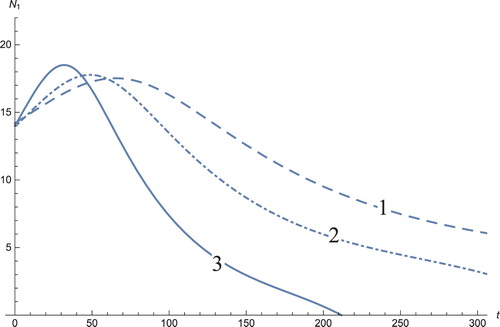
Figure 2. The solution profiles of $N_2\left(t\right)$, the androgen-independent cancer cells. 1: MDDIM, 2: QSS, quasi-steady state approximation, 3: numerical simulations for the full model. These cells decrease rapidly with the onset of immunotherapy.

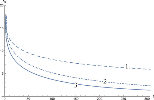
Figure 3. The solutions profiles of the T cells. 1: MDDIM, 2: QSS, quasi-steady state approximation, 3: numerical simulations for the full model. At first treatment, there is a very sharp increase in these cells and then drop to equilibrium point.

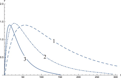
Figure 4. The solution profiles of $I_L\left(t\right)$, the concentration of cytokine. 1: MDDIM, 2: QSS, quasi-steady state approximation, 3: numerical simulations for the full model. During the treatment, the concentration of cytokines increases due to the intense activity of the immune system.

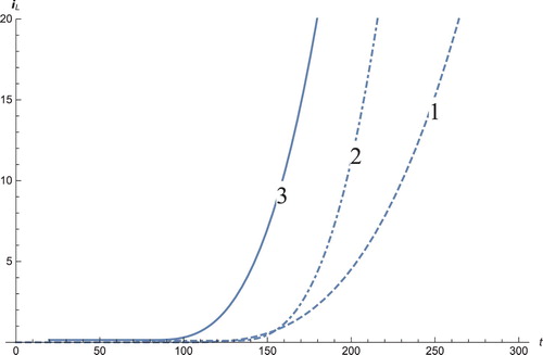
Figure 5. The solution profiles of $A\left(t\right)$, the concentration of androgen. 1: MDDIM, 2: QSS, quasi-steady state approximation, 3: numerical simulations for the full model. The androgens corresponding to the dendritic cells stabilize after ≈60 days, to their equilibrium point.

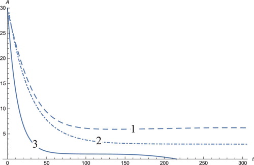
Figure 6. The solution profiles of D, the number of dendritic cells. 1: MDDIM, 2: QSS, quasi-steady state approximation, 3: numerical simulations for the full model. The number of dendritic cells stabilizes after $\approx 56$ days.

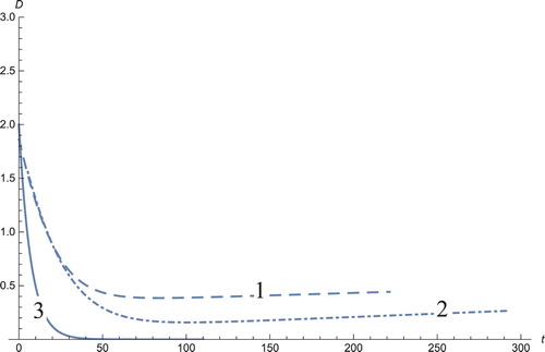
Figure 7. The solution profiles of ${\tilde{N}}_1$, the new variable in the new coordinates. 1: MDDIM, 2: QSS, quasi-steady state approximation, 3: numerical simulations for the full model in the new coordinates, 4: combination of MDDIM and SPVF, 5: SPVF method.

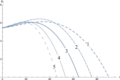
Figure 8. The solution profiles of ${\tilde{N}}_2$, the new variable in the new coordinates. 1: MDDIM, 2: QSS, quasi-steady state approximation, 3: numerical simulations for the full model in the new coordinates, 4: combination of MDDIM and SPVF, 5: SPVF method.

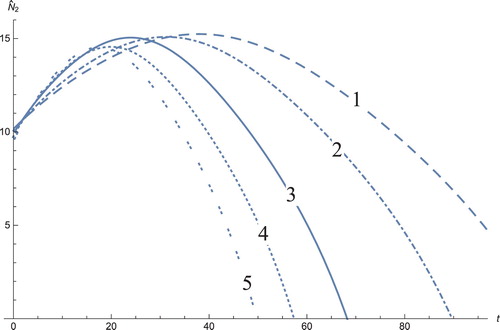
Figure 9. The solution profiles of $\tilde{T}$, the new variable in the new coordinates. 1: MDDIM, 2: QSS, quasi-steady state approximation, 3: numerical simulations for the full model in the new coordinates, 4: combination of MDDIM and SPVF, 5: SPVF method.

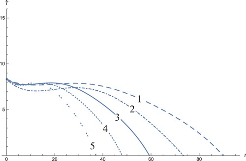
Figure 10. The solution profiles of ${\tilde{I}}_L$, the new variable in the new coordinates. 1: MDDIM, 2: QSS, quasi-steady state approximation, 3: numerical simulations for the full model in the new coordinates, 4: combination of MDDIM and SPVF, 5: SPVF method.

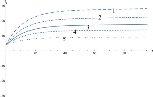
Figure 11. The solution profiles of $\tilde{A}$, the new variable in the new coordinates. 1: MDDIM, 2: QSS, quasi-steady state approximation, 3: numerical simulations for the full model in the new coordinates, 4: combination of MDDIM and SPVF, 5: SPVF method. Since we transfer the model using eigenvectors, we obtain a negative value of $\tilde{A}$ which is biologically insignificant. And hence, for sake of biological understanding, we must ignore these negative values.

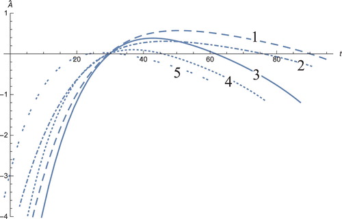
Figure 12. The solution profiles of $\tilde{D}$, the new variable in the new coordinates. 1: MDDIM, 2: QSS, quasi-steady state approximation, 3: numerical simulations for the full model in the new coordinates, 4: combination of MDDIM and SPVF, 5: SPVF method.

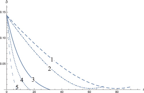
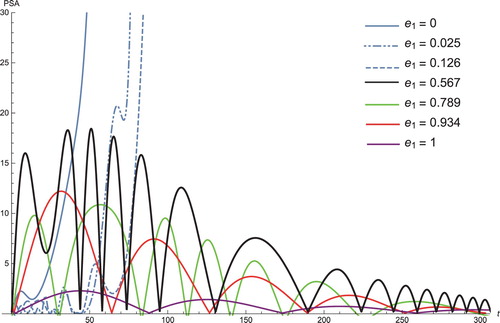
Figure 13. PSA serum level, with an injection rate of 0.078 billion cells for various values of $e_1$, the maximum rate T cells kill cancer cells. A wider range of $e_1$ is able to suppress the growth of cancer and elongate the cycles of IAD.