Cooperative hunting in a discrete predator–prey system II

Figures & data

Figure 1. (a) plots isoclines with four β values to demonstrate Theorem 2.1. (b) provides a graph of $V\left(y\right)$ to illustrate Lemma 2.3. (c) and (d) plot solutions for the case where $y_d<y_t=y_{\ast }$ by removing the first 8000 iterations and plot the next 5000 iterations. In (c), β is chosen larger than $1/\overline{x}$ so that there is a unique interior steady state which is a repeller. In (d), β is smaller than $1/\overline{x}$ but larger than ${\beta }_{\ast }$ so that there are two interior steady states and the boundary steady state $E_1=(\overline{x},0)=(0.5,0)$ is asymptotically stable. The solution converges to the boundary steady state $E_1$.

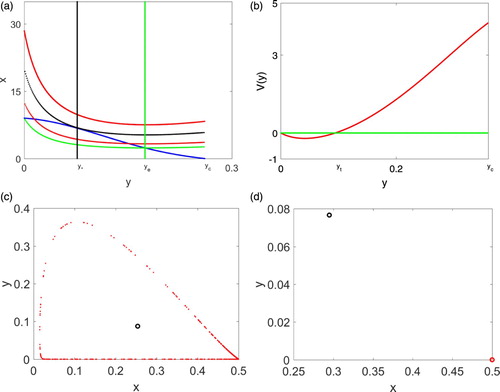
Figure 2. Simulations for the case where $y_{\ast }<y_d$ are presented. In (a) there is a unique interior steady state which is a repeller and the system has an invariant closed curve. In (b)–(d), the system has two attractors and 60,000 randomly generated initial conditions are plotted. Initial conditions convergent to the boundary steady state are denoted by red while initial conditions convergent to the stable interior steady state are marked by blue colour.

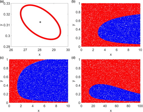
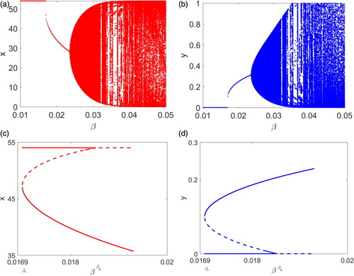
Figure 3. Bifurcation diagrams using β as the varying parameter are presented. (a)–(b) provide attractors of the system and a Neimark–Sacker bifurcation is shown. (c)–(d) plot steady states of the system when β lying in the narrow range $(0.0169962,0.018525)$ where solid and dashed lines denote stable and unstable steady states, respectively. A saddle-node bifurcation at $\beta ={\beta }_{\ast }$ is demonstrated.