Local approximation of Markov chains in time and space

Figures & data

Table 1. State transitions and rates for the single patch CTMC, $X_t$

Description	Transition	Rate
birth ·S	S ↦ $S+1$	$\beta S$
death ·S	S ↦ $S-1$	$\mu S^2$
infection ·I	$S,I$ ↦ S−1,I+1	$S(I+V)$
death ·I	I ↦ $I-1$	$\alpha I$
shed ·V	$I,V$ ↦ $I,V+1$	$\delta I$
clearance ·V	V ↦ $V-1$	$\omega V$

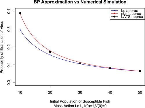
Figure 1. The size of the susceptible population at the disease-free quasistationary distribution is given by $\beta /\mu$. β is the independent variable, while $\mu =1,\alpha =3.3,\delta =1.3,\omega =4$ are fixed. The probability of extinction is approximated using branching process approximation (blue), numerical simulation via Gillespie algorithm (red) and LATS (black).

Table 2. This table illustrates the convergence of entries in the row associated with $x_0$ of ${\mathcal{Q}}_N^N\left(x_0\right)$ to the hitting probabilities $h_{(x_0;X)}\left(E\right)$ and $h_{(x_0;X)}\left(O\right)$.

N	$({\mathcal{Q}}_N^N{)}_{x_{{}_0}e}$	$({\mathcal{Q}}_N^N{)}_{x_{{}_0}o}$	$({\mathcal{Q}}_N^N{)}_{x_{{}_0}g}$
1	0.0154	0	0
10	0.1219	0.0002	0
15	0.1625	0.0028	0
20	0.1945	0.0121	0
25	0.2205	0.0306	0
30	0.2422	0.0582	0
35	0.2609	0.0932	0
40	0.2770	0.1330	0
45	0.2911	0.1752	0
50	0.3035	0.2177	0
100	0.3678	0.5041	0
200	0.3881	0.6048	0
300	0.3892	0.6104	0
400	0.3893	0.6107	0

Notes: For each N, e, o and g are the states in ${\mathcal{S}}_N\left(T\right),$ the state space of the LATS collapsed chain $Y_n$, associated to extinction, outbreak, and escape from the N-neighbourhood, respectively. Parameter values are $\beta =10,\mu =1,\alpha =3.3,\delta =1.3$ and $\omega =4$.

Table 3. This table illustrates the convergence of entries in the row associated with $x_0$ of $H=(I-D{)}^{-1}C$ to the hitting probabilities $h_{(x_0;X)}\left(E\right)$ and $h_{(x_0;X)}\left(O\right)$.

N	$(H{)}_{x_{{}_0}e}$	$(H{)}_{x_{{}_0}o}$	$(H{)}_{x_{{}_0}g}$
1	0.0283	0	0.9717
10	0.3470	0.3645	0.2885
15	0.3892	0.5905	0.0202
20	0.3893	0.6102	0.0005
25	0.3893	0.6107	0
30	0.3893	0.6107	0

Notes: For each N, e, o and g are the states in ${\mathcal{S}}_N\left(T\right),$ the state space of the LATS collapsed chain $Y_n$, associated with extinction, outbreak, and escape from the N-neighbourhood, respectively. The probability of escape does not actually reach 0, but does become so small as to be negligible for the purpose of numerical calculations. Parameter values are the same as those used in Table 2.

Table 4. Patch-specific and overall reproduction numbers for no control, control deployed in patch 1 only and control deployed in patch 2 only.

$({\theta }_1,{\theta }_2)$	${\mathcal{R}}_{01}$	${\mathcal{R}}_{02}$	${\mathcal{R}}_0$
(1,1)	2	5	3.4358
(0.8,1)	1.6	5	3.3146
(1,0.8)	2	4	2.8944

Table 5. State transitions and rates for the two-patch SIS CTMC, $X_t$

Description	Transition	Rate $\sigma (i,j)$
Infection ·$S_1$	$S_1,I_1\mapsto S_1-1,I_1+1$	${\theta }_1{\beta }_1\frac{S_1{I}_1}{N_1}$
Recovery ·$I_1$	$S_1,I_1\mapsto S_1+1,I_1-1$	${\gamma }_1{I}_1$
Infection ·$S_2$	$S_2,I_2\mapsto S_2-1,I_2+1$	${\theta }_2{\beta }_2\frac{S_2{I}_2}{N_2}$
Recovery ·$I_2$	$S_2,I_2\mapsto S_2+1,I_2-1$	${\gamma }_2{I}_2$
Migration ·$S_1$	$S_1,S_2\mapsto S_1-1,S_2+1$	$d{S}_1$
Migration ·$I_1$	$I_1,I_2\mapsto I_1-1,I_2+1$	$d{I}_1$
Migration ·$S_2$	$S_1,S_2\mapsto S_1+1,S_2-1$	$d{S}_2$
Migration ·$I_2$	$I_1,I_2\mapsto I_1+1,I_2-1$	$d{I}_2$

Table 6. Patch i reproduction numbers (${\mathcal{R}}_{0i}$) and GWbp probabilities of extinction (${}^1{/}_{{\mathcal{R}}_{0i}}$) and LATS probabilities of extinction (${\mathbb{P}}_{0i}$) from the initial state $(9,1)$ in patch i=1 and $(4,1)$ in patch i=2 with and without control.

$({\theta }_1,{\theta }_2)$	${\mathcal{R}}_{01}$	${\mathcal{R}}_{02}$	$\frac{1}{{\mathcal{R}}_{01}}$	$\frac{1}{{\mathcal{R}}_{02}}$	${\mathbb{P}}_{01}$	${\mathbb{P}}_{02}$
$(1,1)$	2	5	0.5	0.2	0.5758	0.2727
$(0.8,0.8)$	1.6	4	0.625	0.24	0.6325	0.3439

Note: Parameter values are given by ${\beta }_1=0.4,{\beta }_2=0.5,{\gamma }_1=0.2,{\gamma }_2=0.1,d=0$.

Table 7. Probability of partial extinction in patch 1 only and total extinction from initial state $x_0=(10,1,1,3).$

$({\theta }_1,{\theta }_2)$	$h_{(A;X)}\left(x_0\right)$	$h_{(E;X)}\left(x_0\right)$
(1,1)	0.6157	0.0623
(0.8,1)	0.7095	0.0940
(1,0.8)	0.6591	0.1077

Table 8. The probability of extinction from initial state $x_1=(7,1,7,0)$ and $x_2=(7,0,7,1)$.

$({\theta }_1,{\theta }_2)$	$h_{(x_1;X)}\left(E\right)$	$h_{(x_2;X)}\left(E\right)$
(1,1)	0.5183	0.3298
(0.8,1)	0.5868	0.3602
(1,0.8)	0.5567	0.4151