Optimal control of a vectored plant disease model for a crop with continuous replanting

Figures & data

Figure 1. Compartmental diagram of the abundance-replanting model (2.3(2.1b) $\begin{array}{rl}\frac{\mathrm{d}I}{\mathrm{d}t}& =b\frac{ϵI}{S+ϵI}I\left(1-\frac{N}{\theta }\right)+\beta SW-(\alpha +h+g)I,\end{array}$(2.1b) ). The plant and vector susceptible compartments (Healthy Plants, Non-Infective Vectors) are coloured blue, while their infected compartments (Infected Plants, Infective Vectors) are coloured red. The solid lines indicate the compartment into which a new infection or transfer occurs, while the dotted lines indicate the compartments which are implicitly involved in a given new infection or transfer.

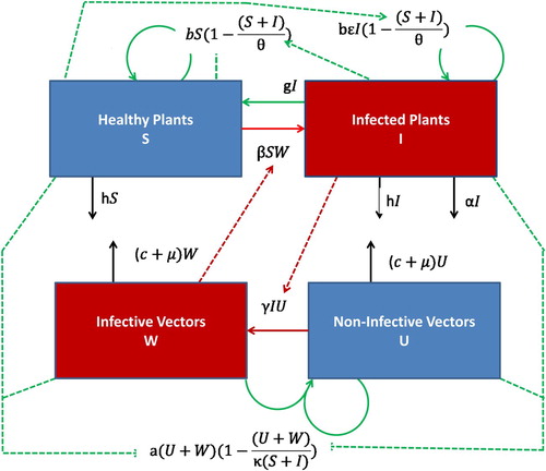
Table 1. Abundance (i.e. density) is measured in numbers per unit area.

Variable	Description
Host
N	Total abundance of host species (N:=S+I)
S	Abundance of healthy plant species
I	Abundance of infected plant species
Vector
V	Total abundance of vectors (V :=U+W)
U	Abundance of non-infective vectors
W	Abundance of infective vectors

Table 2. Parameters and their baseline values as in [14].

Parameter	Description	Range	Baseline Value
Host
b	maximum replanting rate (per day)	$[0.025,0.1]$	0.05
h	harvesting rate (per day)	$[0.002,0.004]$	0.003
r	rate of increase of healthy plant host (r:=b−h)	$[0.023,0.096]$	0.047
α	roguing rate (per day)	$[0,0.033]$	0.003
ε	selection of diseased cuttings for propagation	$[0,1.0]$	0.1
g	recovery rate from infection (per day)	[0.002, 0.004]	0.003
θ	maximum plant population pressure (per m^2)	$[0.01,1.0]$	0.5
K	maximum Host abundance (per m^2) ($K:=r\theta /b$)	$[0.01,1.0]$	0.47
Vector
a	maximum vector birth rate (per day)	$[0.1,0.3]$	0.2
μ	natural vector mortality (per day)	$[0.06,0.18]$	0.06
c	insecticide vector mortality (per day)	$[0,0.18]$	0.06
κ	maximum vector density per host plant	$[0,2500]$	500
$K_v$	maximum vector density (per m${}^2$) ($K_v:=q\kappa K/a$)	$[0,350]$	94
Pathogen
β	vector to host inoculation rate (per vector per day)	$[0.002,0.032]$.	0.008
γ	host to vector acquisition rate (per plant per day)	$[0.002,0.032]$	0.008

Notes: For the roguing rate (α) and insecticide vector mortality (c), the baseline values represent the values used in the sensitivity analysis. For the case of optimal control, where α and c are the control variables, the system is usually started at either equilibrium or non-equilibrium values in the absence of roguing and vector control, i.e. $\alpha =c=0$.

Figure 2. The impact on the abundance at equilibrium of healthy cassava plants (solid line) and infected cassava plants (dashed line) with respect to change in parameters, $c+\mu$ and α. In the top figures α and in the bottom figures c+μ are fixed at their baseline values given in Table 2. The plots in the first column are for the case $ϵ=0$, plots in the middle column are for the case of abundance-replanting with $ϵ=0.1$. The plots in the last column are for frequency-replanting with $ϵ=0.1$.

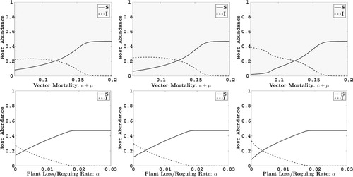
Figure 3. The impact on the abundance at equilibrium of healthy cassava plants (solid line) and infected cassava plants (dashed line) with respect to change in parameters $c+\mu$ and α. In the top figures α, and in the bottom figures c+μ are fixed at their baseline values given in Table 2. The plots in the first column are for the case $ϵ=0$, plots in the middle column are for the case of abundance-replanting with $ϵ=1.0$. The plots in the last column are for frequency-replanting with $ϵ=1.0$.

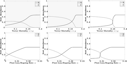
Figure 4. For the abundance-replanting model, the region where the values of the basic reproduction number, ${\mathcal{R}}_{0,A}$, are less than or greater than one are graphed in parameter space as a function of roguing α and vector mortality $c+\mu$ with (Left Plot) $ϵ=0$, (Middle Plot) $ϵ=0.1$, (Right Plot) $ϵ=1.0$. In the frequency-replanting model, ${\mathcal{R}}_{0,F}$ is not dependent on ε. Thus, ${\mathcal{R}}_{0,F}$ is graphed in the left Plot (same for all values of ε).

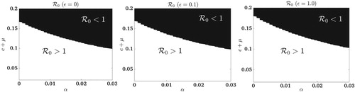
Figure 5. Frequency, equilibrium initial conditions, $ϵ=0.1$: (Top row) Optimal control results for roguing (${\alpha }^{\ast }$) and vector control through insecticides ($c^{\ast }$) for frequency-replanting for the cases of no control, only roguing (α), only vector control through insecticides (c), and roguing and vector control (α and c). (Bottom two rows) Optimally controlled system response in the four cases considered for roguing (${\alpha }^{\ast }$) and vector control ($c^{\ast }$) for frequency-replanting. The cases of roguing (α), insecticide (c), and roguing and insecticide (α and c) combined are contrasted with the uncontrolled system response.

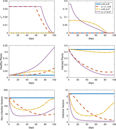
Figure 6. Abundance, equilibrium initial conditions, $ϵ=0.1$: Optimal control results for abundance-replanting for the cases of no control, only roguing (α), only vector control (c), and both roguing and vector control (α and c). Optimally controlled system response in the four cases considered for roguing (${\alpha }^{\ast }$) and vector control ($c^{\ast }$) for abundance-replanting. The cases of roguing (α only), insecticide (c only), and both roguing and insecticide (α and c) combined are contrasted with the uncontrolled system response.

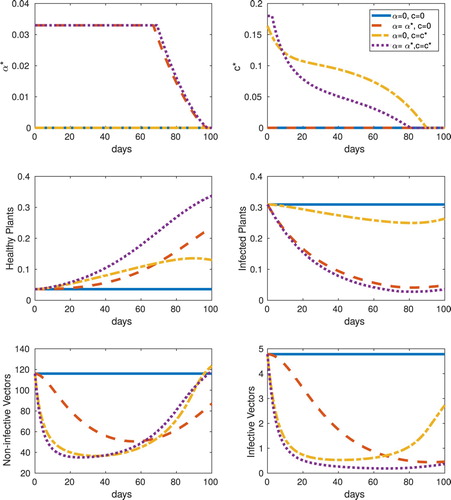
Table 3. Optimal control results for the baseline case.

${\alpha }_{max}$	$c_{max}$	$J\left(F\right)$	$J\left(A\right)$
0	0	0.693	1.205
0.033	0	0.820	2.934
0	0.18	0.793	2.028
0.033	0.18	2.070	4.339

Notes: We consider three types of control strategies, namely, roguing or insecticide use, or both roguing and insecticide use. For each case, we record values of the (optimal) objective functional: $J\left(F\right)$ for frequency-replanting, and $J\left(A\right)$ for abundance-replanting. For reference, the first row is the uncontrolled case. See Figures 5 and 6.

Figure 7. Frequency (top) and abundance (bottom) with equilibrium initial conditions: Optimal controls for different values of the parameter ε. In the results for the abundance-replanting model, as ε increases the optimal control also increase. However, this is not the case in the results for the frequency-replanting model.

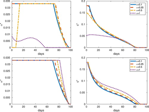
Table 4. Equilibrium solutions for various values of ε for frequency-replanting and abundance-replanting models.

	Frequency-replanting model				Abundance-replanting model
ε	$S_0$	$I_0$	$U_0$	$W_0$	$S_0$	$I_0$	$U_0$	$W_0$
0.1	0.018	0.438	150.966	8.823	0.036	0.309	116.032	4.784
0.25	0.018	0.446	153.304	9.123	0.025	0.374	132.897	6.631
0.5	0.018	0.449	154.049	9.220	0.020	0.423	146.646	8.263
1.0	0.018	0.450	154.416	9.268	0.018	0.452	155.152	9.348

Figure 8. Frequency (top), abundance (bottom), non-equilibrium initial conditions: Optimal controls, ${\alpha }^{\ast }$ and $c^{\ast }$ for different values of ε.

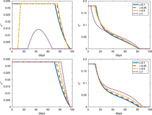
Table 5. Optimal control results for roguing and insecticide control using various values of the selection parameter ε.

	Basic reproduction number		Equilibrium		Non-equilibrium
ε	${\mathcal{R}}_{0,F}$	${\mathcal{R}}_{0,A}$	$J\left(F\right)$	$J\left(A\right)$	$J\left(F\right)$	$J\left(A\right)$
0.1	5.408	5.458	2.070	4.340	2.099	2.845
0.25	5.408	5.533	1.321	3.286	1.404	2.603
0.5	5.408	5.659	0.806	2.584	0.864	2.418
1.0	5.408	5.914	0.728	1.854	0.687	1.885

Notes: For each value of ε, we record the basic reproduction number and the (optimal) objective functional: $J\left(F\right)$ for frequency-replanting, and $J\left(A\right)$ for abundance type replanting. Equilibrium and non-equilibrium initial conditions are compared.

Figure A1. Graphs of $F_1(S,I)=0$ (dashed curve) and $F_2(S,I)=0$ (solid curve), given by Equations (3.9a(3.9a) $\begin{array}{rl}{F}_1(S,I)& =b\frac{S^2+ϵI^2}{S+ϵI}\left(1-\frac{N}{\theta }\right)-hN-\alpha I=0,\end{array}$(3.9a) )–(3.9b(3.9b) $\begin{array}{rl}{F}_2(S,I)& =\frac{bϵI}{S+ϵI}\left(1-\frac{N}{\theta }\right)+\frac{\beta \kappa q\gamma SN}{a(\gamma I+\mu +c)}-(\alpha +h+g)=0,\end{array}$(3.9b) ), for the baseline parameter values in Table 2, except $ϵ=1$ and α. The α values and the EE in (a) $\alpha =0.007$, $(S^{\ast },I^{\ast })=(0.3005,0.0734)$, (b) $\alpha =0.008$, $(S^{\ast },I^{\ast })=(0.1502,0.2325),$ $(0.1961,0.1568)$, and $(0.2766,0.0817)$, (c) $\alpha =0.009$, $(S^{\ast },I^{\ast })=(0.1186,0.2848)$, and (d) $\alpha =0.01$, $(S^{\ast },I^{\ast })=(0.0982,0.3179).$ In (a)–(d), there exists a unique locally stable EE (blue circle) but in (b), there exist two locally stable EE (blue circle) separated by an unstable EE (green asterisk). Note the change in shape of the curve $F_2(S,I)=0$ when α increases from 0.007 in (a) to 0.008 in (b).

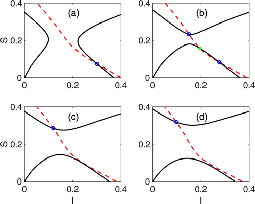
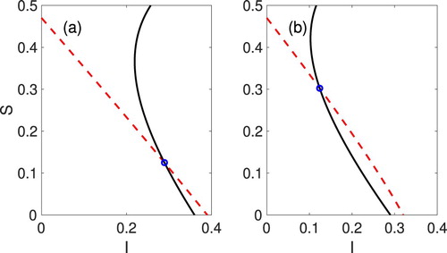
Figure A2. Graphs of $G_1(S,I)=0$ (dashed curve) and $G_2(S,I)=0$ (solid curve), given by Equations (3.10a(3.10a) $\begin{array}{rl}{G}_1(S,I)& =b(S+ϵI)\left(1-\frac{N}{\theta }\right)-hN-\alpha I=0,\end{array}$(3.10a) )–(3.10b(3.10b) $\begin{array}{rl}{G}_2(S,I)& =bϵ\left(1-\frac{N}{\theta }\right)+\frac{\beta \kappa q\gamma SN}{a(\gamma I+\mu +c)}-(\alpha +h+g)=0.\end{array}$(3.10b) ), for all of the baseline parameter values in Table 2, except for $ϵ=1$ and α. The α values and the locally stable EE (blue circle) in (a) $\alpha =0.008$, $(S^{\ast },I^{\ast })=(0.2892,0.1249)$ and (b) $\alpha =0.015$, $(S^{\ast },I^{\ast })=(0.1240,0.3023)$.

J. Holt, M.J. Jeger, J.M. Thresh and G.W. Otim-Nape, An epidemiological model incorporating vector population dynamics applied to African cassava mosaic virus disease, J. Appl. Ecol. 34 (1997), pp. 793–806. doi: 10.2307/2404924

 Web of Science ®Google Scholar