Figures & data
Figure 1. EIL: the lowest population density that will cause economic damage. ET: population density at which control measures should be invoked to prevent an increasing pest population from reaching EIL.
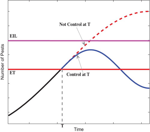
Figure 2. The two real branches and
of Lambert W function.
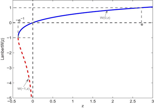
Figure 3. Bifurcation diagram for the existence of regular equilibria of system (Equation5(5)
(5) ) with respect to r and ET, parameters are
.
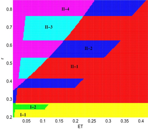
Figure 4. Bifurcation diagram for system (Equation5(5)
(5) ) with respect to r. All other parameters as follows:
and
.
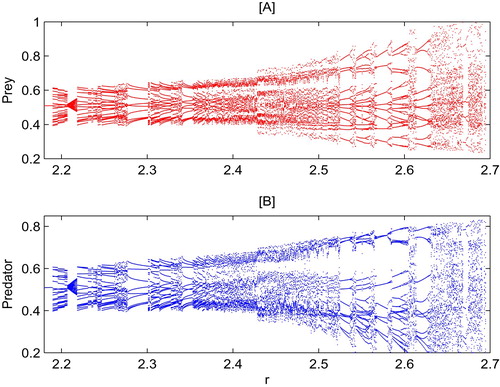
Figure 5. Phase-plan of system (Equation5(5)
(5) ) with different r. [A] r = 2.18; [B] r = 2.213; [C] r = 2.4; [D] r = 2.65. The other parameters are identical to those in Figure .
![Figure 5. Phase-plan of system (Equation5(5) Z˙(t)={FS1(Z),Z∈S1,FS2(Z),Z∈S2,(5) ) with different r. [A] r = 2.18; [B] r = 2.213; [C] r = 2.4; [D] r = 2.65. The other parameters are identical to those in Figure 4.](/cms/asset/070dbf1d-0c34-44ee-90e6-19ccad3e9887/tjbd_a_1682200_f0005_oc.jpg)
Figure 6. Bifurcation diagram for system (Equation5(5)
(5) ) with respect to q. All other parameters as follows:
, and [A]
; [B]
; [C]
.
![Figure 6. Bifurcation diagram for system (Equation5(5) Z˙(t)={FS1(Z),Z∈S1,FS2(Z),Z∈S2,(5) ) with respect to q. All other parameters as follows: a=1.68,ET=0.72,r=2.58,(H0,P0)=(0.1,0.1), and [A] θ=9.5; [B] θ=5; [C] θ=1.](/cms/asset/a7fd62d6-4ced-4e6a-a23b-2bd70bb84742/tjbd_a_1682200_f0006_oc.jpg)
Figure 7. Bifurcation diagram for system (Equation5(5)
(5) ) with respect to θ. All other parameters as follows:
, and [A] r = 2.13; [B] r = 2.
![Figure 7. Bifurcation diagram for system (Equation5(5) Z˙(t)={FS1(Z),Z∈S1,FS2(Z),Z∈S2,(5) ) with respect to θ. All other parameters as follows: a=2,q=0.8,ET=0.8,r=2.29,(H0,P0)=(0.3,0.2), and [A] r = 2.13; [B] r = 2.](/cms/asset/03d0b846-e5f8-444a-8608-b85eb57fe996/tjbd_a_1682200_f0007_oc.jpg)
Figure 8. Switching effect of system (Equation5(5)
(5) ) under different initial densities. Parameters are
.
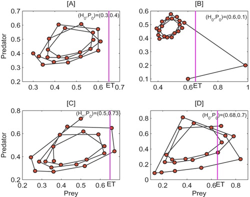
Figure 9. Pest outbreak frequency depends on initial density of system (Equation5
(5)
(5) ). The parameters are fixed as
.
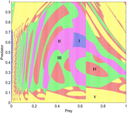
Figure 10. The coexisting attractors of system (Equation5(5)
(5) ) with different initial values. Parameters are
, and [A]
; [B]
.
![Figure 10. The coexisting attractors of system (Equation5(5) Z˙(t)={FS1(Z),Z∈S1,FS2(Z),Z∈S2,(5) ) with different initial values. Parameters are a=2,θ=4,q=0.05,ET=0.45,r=2.3, and [A] (H0,P0)=(0.6,0.4); [B] (H0,P0)=(0.1,0.1).](/cms/asset/faff0f16-3dee-4174-bfaa-3a83b963ec38/tjbd_a_1682200_f0010_oc.jpg)
Figure 11. Basin of attraction of two attractors shown in Fig. with and
. The white and black points are attracted to the attractors shown in Figure from left to right.
![Figure 11. Basin of attraction of two attractors shown in Fig. 10 with H∈[0.3,0.67] and P∈[0.2,0.8]. The white and black points are attracted to the attractors shown in Figure 10 from left to right.](/cms/asset/f6e3ae38-b57b-4045-8477-90d2df92dbd0/tjbd_a_1682200_f0011_ob.jpg)
Figure 12. Attractors' switch-like behavior of system (Equation5(5)
(5) ) with
has random perturbation as each 90 generations. Parameters are:
and
.
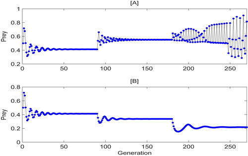
Figure 13. Attractors' switch-like behavior of system (Equation5(5)
(5) ) with
which random perturbation every 90 generations. Parameters are:
and
.
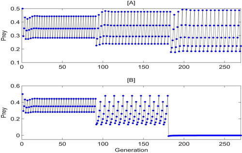
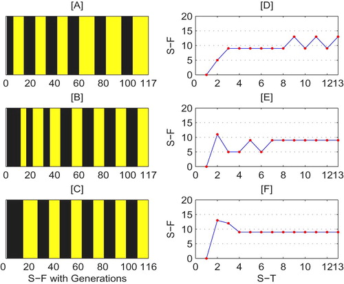
Figure 14. Switching frequency (S-F) and switching time (S-T) of system (Equation5(5)
(5) ). Parameters are
. The initial densities from top to bottom are
and
.