Stability of a certain class of a host–parasitoid models with a spatial refuge effect

Figures & data

Figure 1. Trajectories (black) and approximated invariant curve (red) for a = 0.5, m = 1.5, c = 1.0, $b_0=1.5$ and b = 1.45, b = 1.49 b = 1.495, b = 1.5, b = 1.53, b = 1.7, respectively for $\left(S\right)$ model.

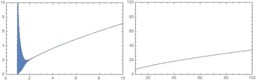
Figure 2. Bifurcation diagrams in b−P plane for a = 0.5, c = 1.0, and m = 1.5 for $\left(S\right)$ model.

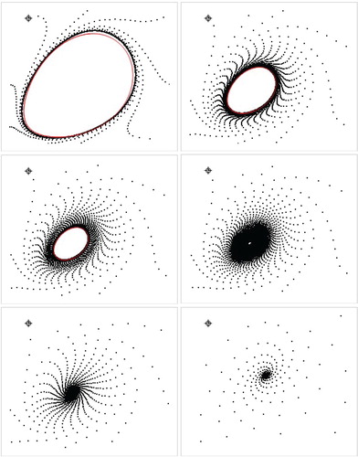
Figure 3. Bifurcation diagrams in b−P plane for a = 0.1, c = 1.0. and m = 0.4 for $\left(HV\right)$ model.

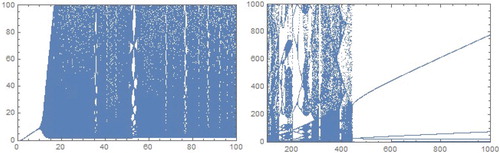
Figure 4. The corresponding regions of (a) stability (b) Hopf border surface and (c) instability in a−m−b space for $\left(HV\right)$.

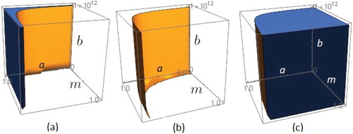
Figure 5. Graphs of the functions $\alpha \left(b_0\right)\left(m\right)$ and $d\left(b_0\right)\left(m\right)$ for some values of a for $\left(HV\right)$ model.

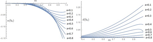
Figure 6. Trajectories (black) and approximated invariant curve (red) for a = 0.1, m = 0.4, c = 1.0, $b_0\approx 11.358951291565068$ and b = 11.239, b = 11.349 $b=b_0$, b = 11.36, b = 11.37, b = 11.48, respectively, for $\left(HV\right)$.

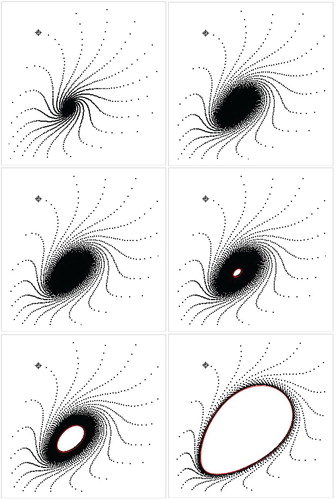
Table 1. The coefficients $b_0$, $d\left(b_0\right)$, and $\alpha \left(b_0\right)$ for some values of a, m and c = 1.

a	m	$b_0$	$d\left(b_0\right)$	$\alpha \left(b_0\right)$
0.2	0.2	408.115	0.000193498	$-8.41286\times {10}^{-10}$
0.3	0.2	878.357	0.0000791367	$-4.12591\times {10}^{-10}$
$0.4$	$0.2$	$2487.81$	$0.0000240465$	$-1.57987\times {10}^{-10}$
$0.2$	$0.3$	$47.2634$	$0.00236688$	$-6.27282\times {10}^{-6}$
$0.3$	$0.3$	$76.9854$	$0.00129697$	$-4.51672\times {10}^{-6}$
$0.4$	$0.3$	$149.558$	$0.00058343$	$-2.78057\times {10}^{-6}$
$0.5$	$0.3$	$386.17$	$0.000191366$	$-1.45415\times {10}^{-6}$
0.6	$0.3$	$1655.75$	$0.0000360768$	$-6.17268\times {10}^{-7}$
0.7	$0.3$	20062.	$2.24191\times {10}^{-6}$	$-1.91295\times {10}^{-7}$
0.8	$0.3$	$3.46154\times {10}^6$	$8.66663\times {10}^{-9}$	$-3.37687\times {10}^{-8}$
0.2	$0.4$	$14.7794$	0.00921253	$-0.000322423$
0.3	$0.4$	$21.0644$	0.00582341	$-0.000276712$
0.4	$0.4$	$34.3241$	0.00317278	$-0.000212010$
0.5	$0.4$	$69.0598$	0.0013643	$-0.000145720$
0.6	$0.4$	$200.876$	$0.000387863$	$-0.0000879042$
0.7	$0.4$	$1239.72$	$0.0000481118$	$-0.0000436707$
0.8	$0.4$	53655.	$7.45345\times {10}^{-7}$	$-0.0000152052$
0.2	$0.5$	$6.82909$	0.0223457	$-0.00272459$
0.3	$0.5$	$8.94916$	0.0153722	$-0.00259559$
0.4	$0.5$	$13.1514$	0.00937468	$-0.00225813$
0.5	$0.5$	$23.0316$	0.00472516	$-0.00181520$
0.6	$0.5$	$54.1873$	$0.00171009$	$-0.00133904$
0.7	$0.5$	$228.988$	0.000319442	$-0.000875038$
0.8	$0.5$	$4395.28$	0.0000113525	$-0.000456443$
0.2	$0.6$	$3.83278$	0.0423834	$-0.00984863$
0.3	$0.6$	$4.70446$	0.0308358	$-0.0101025$
0.4	$0.6$	$6.42245$	0.0202532	$-0.00958838$
0.5	$0.6$	$10.2912$	0.0113319	$-0.00855720$
0.6	$0.6$	$21.3369$	$0.00480405$	$-0.00720453$
0.7	$0.6$	$71.8832$	0.00117329	$-0.00563043$
0.8	$0.6$	$823.685$	0.0000721954	$-0.00383243$
0.2	$0.7$	$2.40189$	0.0693849	$-0.0221926$
0.3	$0.7$	$2.77369$	0.0524804	$-0.0241553$
0.4	$0.7$	$3.55315$	0.0362865	$-0.0245286$
0.5	$0.7$	$5.33549$	0.0218627	$-0.0236906$
0.6	$0.7$	$10.2306$	0.0103803	$-0.0220000$
0.7	$0.7$	$30.0575$	0.00306441	$-0.0195813$
0.8	$0.7$	$245.784$	0.000277706	$-0.0161163$
0.2	$0.8$	$1.60905$	$0.103068$	$-0.0369197$
0.3	$0.8$	$1.73865$	0.0799625	$-0.0423442$
0.4	$0.8$	$2.08061$	0.0571231	$-0.0455823$
0.5	$0.8$	$2.95318$	0.0363071	$-0.0470695$
0.6	$0.8$	$5.41502$	0.018864	$-0.0474562$
0.7	$0.8$	$14.7851$	0.00644749	$-0.0469722$
0.8	$0.8$	$97.2016$	0.000778919	$-0.0447984$

Figure 7. The corresponding regions of (a) stability (b) Hopf border surface and (c) instability in a−m−b space for $\left(PP\right)$ model.

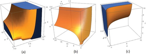
Figure 8. Bifurcation diagrams in b−P plane for a = 0.01, c = 1.0. and $m_0=6.040735644332293$ for $\left(PP\right)$ model.

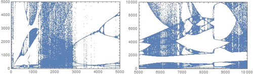
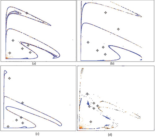
Figure 9. Supercritical Hopf bifurcation for a = 0.01, m = 10, c = 1 where $b_0\approx 4.213439215488374$, $d\left(b_0\right)\approx 0.040557714674268774$, and $\alpha \left(b_0\right)\approx -8.53863\times {10}^{-7}$. Trajectories (orange, blue and black) and approximated attractive invariant curve (red) for (a) b = 4.2 (b) b = 4.214 (c) b = 4.22 and (d) b = 4.225. For $\left(PP\right)$ model.

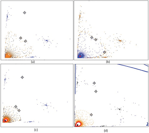
Figure 10. Supercritical Hopf bifurcation for a = 0.1, m = 10, c = 1 where $b_0\approx 4.803161528187171$, $d\left(b_0\right)\approx 0.03290632603362123$, and $\alpha \left(b_0\right)\approx -2.10776\times {10}^{-7}$. Trajectories (orange, blue and black) and approximated attractive invariant curve (red) for (c) b = 4.81 and (d) b = 4.88 and trajectories for (a) b = 4.6 and (b) b = 4.8. For$\left(PP\right)$ model.

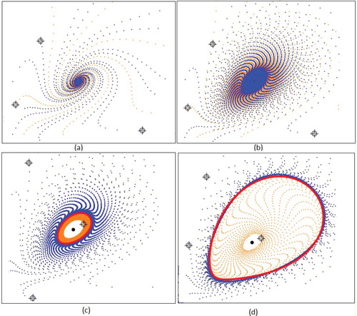
Figure 11. Subcritical Hopf bifurcation for a = 0.1, m = 1.8, c = 1 where $b_0\approx 2.381196753601008$, $d\left(b_0\right)\approx 0.043144048585692873$, and $\alpha \left(b_0\right)\approx 0.00010912518875029679$. Trajectories (orange, blue and black) and approximated repelling invariant curve (red) for (a) b = 2.37 and (b) b = 2.38 and trajectories for (c) b = 2.382 and (b) b = 2.39. For $\left(PP\right)$ model.

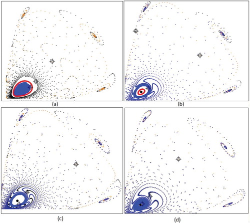
Table 2. The coefficients $b_0$, $d\left(b_0\right)$, and $\alpha \left(b_0\right)$ for some values of a, m and c = 1.

a	m	$b_0$	$d\left(b_0\right)$	$\alpha \left(b_0\right)$
0.01	$1.1$	$1.16932$	$0.0221388$	$0.0191121$
0.01	$2.1$	$2.28577$	0.0489982	$0.000334622$
0.01	$3.1$	$2.92481$	$0.0470603$	$0.000029227$
0.01	$4.1$	$3.32418$	$0.0450936$	$4.31592\times {10}^{-6}$
0.01	5.1	$3.59515$	$0.0436907$	$6.6182\times {10}^{-7}$
0.01	$6.1$	$3.79047$	0.0426817	$-1.63676\times {10}^{-8}$
0.05	$1.1$	$1.27047$	$0.0309502$	0.010163
0.05	$2.1$	$2.44035$	$0.0462047$	$0.000160244$
0.05	$3.1$	3.10621	$0.0435757$	$8.35346\times {10}^{-6}$
0.05	$4.1$	$3.52148$	0.0415353	$-6.04233\times {10}^{-7}$
0.05	$5.1$	$3.80292$	0.040149	$-9.90726\times {10}^{-7}$
0.05	$6.1$	$4.00566$	0.0391716	$-7.0604\times {10}^{-7}$
0.1	$1.1$	$1.42955$	$0.0369549$	0.00394312
0.1	$2.1$	$2.6814$	$0.0421882$	$0.0000197167$
0.1	$3.1$	3.38858	$0.039053$	$-9.10164\times {10}^{-6}$
0.1	$4.1$	$3.82837$	0.0370162	$-4.78208\times {10}^{-6}$
0.1	$5.1$	$4.12599$	0.0356905	$-2.40488\times {10}^{-6}$
0.1	$6.1$	$4.34019$	0.0347731	$-1.29881\times {10}^{-6}$
0.15	$1.1$	$1.63731$	$0.038771$	0.000786658
0.15	$2.1$	$2.99319$	$0.0377399$	$-0.0000623552$
0.15	3.1	$3.75297$	$0.0344211$	$-0.0000196141$
0.15	$4.1$	$4.22403$	0.0324749	$-7.32143\times {10}^{-6}$
0.15	$5.1$	$4.5423$	0.0312456	$-3.26624\times {10}^{-6}$
0.15	$6.1$	$4.77114$	0.0304067	$-1.65959\times {10}^{-6}$

Figure 12. Trajectories (orange, blue and black) for a = 0.01, $b_0\approx 3.780433954506987$, c = 1 where $m_0\approx 6.040735644332293$, and $\alpha \left(b_0\right)\approx 0$ for (a) b = 3.25, $m=m_0$ (b) b = 3.87, $m=m_0$ (c) $b=b_0$, m = 3.72 and (d) $b=b_0$, m = 8.97. for $\left(PP\right)$ model.