A stochastic SACR epidemic model for HBV transmission

Figures & data

Table 1. Parameters value.

Notation	Parameter description	Value	Source
b	The constant birth rate	0.5	[11]
α	The transmission rate	0.6, 0.36 ${\mathrm{d}\mathrm{a}\mathrm{y}}^{-1}$	[11]
${\mu }_0$	Natural death rate	0.5	[11]
${\mu }_1$	The disease induced death rate	0.2 ${\mathrm{d}\mathrm{a}\mathrm{y}}^{-1}$	[11]
v	The vaccination rate	0.01	[11]
${\gamma }_1$	The constant recovery rate for acutely infected individuals	0.2, 0.4 ${\mathrm{d}\mathrm{a}\mathrm{y}}^{-1}$	[11]
${\gamma }_2$	The constant recovery rate for chronically infected individuals	0.4, 0.2 ${\mathrm{d}\mathrm{a}\mathrm{y}}^{-1}$	[11]
β	The moving rate of acutely infected individuals to chronic stage	0.1, 0.4 ${\mathrm{d}\mathrm{a}\mathrm{y}}^{-1}$	[11]

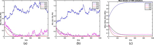
Figure 1. For the verification of the hepatitis B extinction i.e.  Theorem 4.1, we assume the parameter values as: b = 0.5, $\text{β}=0.1$, ${\text{β}}_2=0.5$, ${\mu }_0=0.5$, v = 0.01, ${\gamma }_1=0.2$, ${\gamma }_2=0.4$, ${\mu }_1=0.2$, $\sigma =0.5$. It is easy to ensure the condition (a) i.e. $R_0=\mathrm{0.0.734729}<1$, $\alpha ({\mu }_0+v)=0.306>0.125={\sigma }^{2}b$. This indicates the extinction of the hepatitis B. On the other hand, for the corresponding deterministic model (2(2) $\begin{array}{rl}\mathrm{d}S\left(t\right)& =(b-\alpha S\left(t\right)C\left(t\right)-(v+{\mu }_0)S\left(t\right))\mathrm{d}t,\\ \mathrm{d}A\left(t\right)& =(\alpha S\left(t\right)C\left(t\right)-({\gamma }_1+{\mu }_0+\text{β})A\left(t\right))\mathrm{d}t,\\ \mathrm{d}C\left(t\right)& =(\text{β}A\left(t\right)-({\gamma }_2+{\mu }_0+{\mu }_1)C\left(t\right))\mathrm{d}t,\\ \mathrm{d}R\left(t\right)& =vS\left(t\right)+({\gamma }_{2}C\left(t\right)-{\mu }_{0}R\left(t\right)+{\gamma }_{1}A\left(t\right))\mathrm{d}t.\end{array}$(2) ), $R_0^d=1.2$ then the endemic equilibrium ($S^{\ast },A^{\ast },C^{\ast },R^{\ast }$) is globally asymptotically stable. (a) Test 1: Realization 1 with time in days. (b) Test 1: Realization 2 with time in days. (c) Test 1: Mean Solution with time in days.

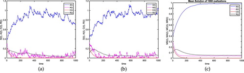
Figure 2. The plot shows the extinction of the proposed model $\left(1\right)$ for $\sigma =0.35$. Comparing with Figure (1), with the noise getting smaller, the fluctuation of the solution of system (1(1) $\begin{array}{rl}\mathrm{d}S\left(t\right)& =(b-\alpha S\left(t\right)C\left(t\right)-(v+{\mu }_0)S\left(t\right))\mathrm{d}t-\sigma S\left(t\right)C\left(t\right)\mathrm{d}B\left(t\right),\\ \mathrm{d}A\left(t\right)& =(\alpha S\left(t\right)C\left(t\right)-({\gamma }_1+{\mu }_0+\text{β})A\left(t\right))\mathrm{d}t+\sigma S\left(t\right)C\left(t\right)\mathrm{d}B\left(t\right),\\ \mathrm{d}C\left(t\right)& =(\text{β}A\left(t\right)-({\gamma }_2+{\mu }_0+{\mu }_1)C\left(t\right))\mathrm{d}t,\\ \mathrm{d}R\left(t\right)& =vS\left(t\right)+({\gamma }_{2}C\left(t\right)-{\mu }_{0}R\left(t\right)+{\gamma }_{1}A\left(t\right))\mathrm{d}t.\end{array}$(1) ) is getting weaker. (a) Test 2: Realization 1 with time in days. (b) Test 2: Realization 2 with time in days. (c) Test 2: Mean Solution with time in days.

Table 2. List of parameters.

	Test 1	Test 2
$C_0$	1.3	1.3
$R_0$	0.5	0.5
$A_0$	0.8	0.8
$S_0$	0.3	0.3
$C_s$	1.3461	1.3461
$R_s$	0.5121	0.5121
$A_s$	0.1513	0.1513
$S_s$	0.9246	0.9246
${\mu }_1$	0.2	0.2
${\mu }_0$	0.5	0.5
${\gamma }_1$	0.2	0.4
${\gamma }_2$	0.4	0.2
b	0.5	0.5
α	0.60	0.360
v	0.01	0.01
β	0.1	0.4
σ	0.5	0.35

T. Khan, A. Khan, and G. Zaman, The extinction and persisitence of the stochastic hepatitis B epidemic model, Chaos. Sol. Fractals 108 (2018), pp. 123–128. doi: 10.1016/j.chaos.2018.01.036

 Web of Science ®Google Scholar