1,080
Views
15
CrossRef citations to date
0
Altmetric
2019 Guangzhou Workshop

Survival analysis of a stochastic predator–prey model with prey refuge and fear effect

&
Pages 871-892 | Received 14 Jan 2020, Accepted 10 Nov 2020, Published online: 03 Dec 2020

Figures & data

Figure 1. (a) and (c): The asymptotic behaviour of the solutions to stochastic model (2) around the positive equilibrium of model (1) with initial value (x(0),y(0))=(0.6,0.5); (b) and (d): The density function diagrams of x(t) and y(t), respectively. The parameters are taken as (Equation23) and m = 0.1, K = 0.3, σ1=σ2=0.01.

Figure 1. (a) and (c): The asymptotic behaviour of the solutions to stochastic model (2) around the positive equilibrium of model (1) with initial value (x(0),y(0))=(0.6,0.5); (b) and (d): The density function diagrams of x(t) and y(t), respectively. The parameters are taken as (Equation23(23) α=0.6,b=0.3,β=0.3,c=0.8,a=0.3,γ=0.1,(23) ) and m = 0.1, K = 0.3, σ1=σ2=0.01.

Figure 2. Numerical simulation for model (Equation1) and model (Equation2) with initial value (x(0),y(0))=(0.6,0.5). The parameters are taken as (Equation23) and m = 0.1, K = 0.3, σ1=1.1, σ2=0.01.

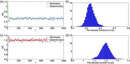
Figure 2. Numerical simulation for model (Equation1(1) dxdt=αx1+Ky−bx2−β(1−m)xy1+a(1−m)x,dydt=−γy+cβ(1−m)xy1+a(1−m)x,(1) ) and model (Equation2(2) dx=αx1+Ky−bx2−β(1−m)xy1+a(1−m)xdt+σ1xdB1(t),dy=−γy+cβ(1−m)xy1+a(1−m)xdt+σ2ydB2(t),(2) ) with initial value (x(0),y(0))=(0.6,0.5). The parameters are taken as (Equation23(23) α=0.6,b=0.3,β=0.3,c=0.8,a=0.3,γ=0.1,(23) ) and m = 0.1, K = 0.3, σ1=1.1, σ2=0.01.

Figure 3. Numerical simulation for model (Equation1) and model (Equation2) with initial value (x(0),y(0))=(0.6,0.5). The parameters are taken as (Equation23) and m = 0.1, K = 0.3, σ1=0.1, σ2=0.9.

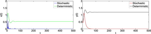
Figure 3. Numerical simulation for model (Equation1(1) dxdt=αx1+Ky−bx2−β(1−m)xy1+a(1−m)x,dydt=−γy+cβ(1−m)xy1+a(1−m)x,(1) ) and model (Equation2(2) dx=αx1+Ky−bx2−β(1−m)xy1+a(1−m)xdt+σ1xdB1(t),dy=−γy+cβ(1−m)xy1+a(1−m)xdt+σ2ydB2(t),(2) ) with initial value (x(0),y(0))=(0.6,0.5). The parameters are taken as (Equation23(23) α=0.6,b=0.3,β=0.3,c=0.8,a=0.3,γ=0.1,(23) ) and m = 0.1, K = 0.3, σ1=0.1, σ2=0.9.

Figure 4. Numerical simulation for model (Equation1) and model (Equation2) with initial value (x(0),y(0))=(0.6,0.5) and different K, respectively. The parameters are taken as (Equation23) and m = 0.1, σ1=σ2=0.01.

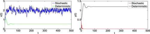
Figure 4. Numerical simulation for model (Equation1(1) dxdt=αx1+Ky−bx2−β(1−m)xy1+a(1−m)x,dydt=−γy+cβ(1−m)xy1+a(1−m)x,(1) ) and model (Equation2(2) dx=αx1+Ky−bx2−β(1−m)xy1+a(1−m)xdt+σ1xdB1(t),dy=−γy+cβ(1−m)xy1+a(1−m)xdt+σ2ydB2(t),(2) ) with initial value (x(0),y(0))=(0.6,0.5) and different K, respectively. The parameters are taken as (Equation23(23) α=0.6,b=0.3,β=0.3,c=0.8,a=0.3,γ=0.1,(23) ) and m = 0.1, σ1=σ2=0.01.

Figure 5. The solutions of model (Equation2) with the initial value (x(0),y(0))=(0.6,0.5) and different K,m, respectively. The parameters are taken as (Equation23) and σ1=σ2=0.01.

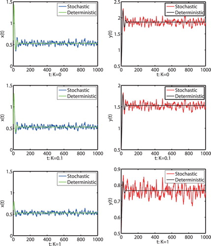
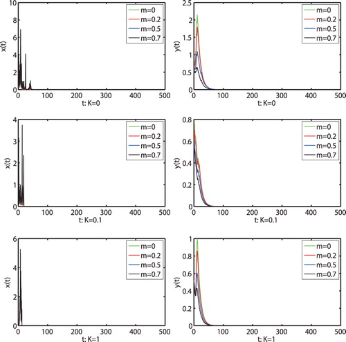
Figure 5. The solutions of model (Equation2(2) dx=αx1+Ky−bx2−β(1−m)xy1+a(1−m)xdt+σ1xdB1(t),dy=−γy+cβ(1−m)xy1+a(1−m)xdt+σ2ydB2(t),(2) ) with the initial value (x(0),y(0))=(0.6,0.5) and different K,m, respectively. The parameters are taken as (Equation23(23) α=0.6,b=0.3,β=0.3,c=0.8,a=0.3,γ=0.1,(23) ) and σ1=σ2=0.01.

Figure 6. The solutions of model (Equation2) with the initial value (x(0),y(0))=(0.6,0.5) and different K,m, respectively. The parameters are taken as (Equation23) and σ1=1.1,σ2=0.01.

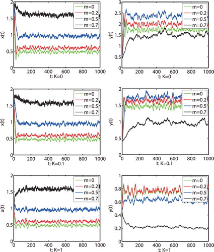
Figure 6. The solutions of model (Equation2(2) dx=αx1+Ky−bx2−β(1−m)xy1+a(1−m)xdt+σ1xdB1(t),dy=−γy+cβ(1−m)xy1+a(1−m)xdt+σ2ydB2(t),(2) ) with the initial value (x(0),y(0))=(0.6,0.5) and different K,m, respectively. The parameters are taken as (Equation23(23) α=0.6,b=0.3,β=0.3,c=0.8,a=0.3,γ=0.1,(23) ) and σ1=1.1,σ2=0.01.