Evaluating different epidemiological models with the identical basic reproduction number ℛ₀

Figures & data

Figure 1. The uniqueness of the final epidemic size, with respect to the basic reproduction number ${\mathcal{R}}_0$.

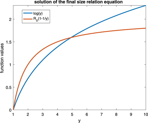
Figure 2. The x-axis represents time (in days) and the y-axis represents the numbers of individuals in different compartments with respect to time. Outbreaks are initiated by one infectious individual. Plots on lower left and on lower right represent the sums of $S_1+S_2$, $I_1+I_2$ and $R_1+R_2$ for models (12(12) $\begin{array}{rl}{S}_1^{\mathrm{\prime }}& =-S_1[p_{11}{\beta }_1{\displaystyle \frac{I_1}{N_1}}+p_{12}{\beta }_1{\displaystyle \frac{I_2}{N_2}}],\\ I_1^{\mathrm{\prime }}& =S_1[p_{11}{\beta }_1{\displaystyle \frac{I_1}{N_1}}+p_{12}{\beta }_1{\displaystyle \frac{I_2}{N_2}}]-\gamma I_1,\\ R_1^{\mathrm{\prime }}& =\gamma I_1,\\ S_2^{\mathrm{\prime }}& =-S_2[p_{21}{\beta }_2{\displaystyle \frac{I_1}{N_1}}+p_{22}{\beta }_2{\displaystyle \frac{I_2}{N_2}}],\\ I_2^{\mathrm{\prime }}& =S_2[p_{21}{\beta }_2{\displaystyle \frac{I_1}{N_1}}+p_{22}{\beta }_2{\displaystyle \frac{I_2}{N_2}}]-\gamma I_2,\\ R_2^{\mathrm{\prime }}& =\gamma I_2.\end{array}$(12) ) and (19(19) $\begin{array}{rl}{S}_1^{\mathrm{\prime }}& =-S_1{a}_1(t)[p_1{\displaystyle \frac{I_1}{N_1}}+p_2{\displaystyle \frac{I_2}{N_2}}],\\ I_1^{\mathrm{\prime }}& =S_1{a}_1(t)[p_1{\displaystyle \frac{I_1}{N_1}}+p_2{\displaystyle \frac{I_2}{N_2}}]-\gamma I_1,\\ R_1^{\mathrm{\prime }}& =\gamma I_1,\\ S_2^{\mathrm{\prime }}& =-S_2{a}_2(t)[p_1{\displaystyle \frac{I_1}{N_1}}+p_2{\displaystyle \frac{I_2}{N_2}}],\\ I_2^{\mathrm{\prime }}& =S_2{a}_2(t)[p_1{\displaystyle \frac{I_1}{N_1}}+p_2{\displaystyle \frac{I_2}{N_2}}]-\gamma I_2,\\ R_2^{\mathrm{\prime }}& =\gamma I_2.\end{array}$(19) ), respectively.

Table 1. The final epidemic sizes for epidemic models (3(3) $\begin{array}{l}{S}^{\mathrm{\prime }}=-\beta S{\displaystyle \frac{I}{N}},\\ I^{\mathrm{\prime }}=\beta S{\displaystyle \frac{I}{N}}-\gamma I,\\ R^{\mathrm{\prime }}=\gamma I.\end{array}$(3) ), (7(7) $\begin{array}{rl}{S}^{\mathrm{\prime }}& =-a(t)S{\displaystyle \frac{I}{N}},\\ I^{\mathrm{\prime }}& =a(t)S{\displaystyle \frac{I}{N}}-\gamma I,\\ R^{\mathrm{\prime }}& =\gamma I.\end{array}$(7) ), (12(12) $\begin{array}{rl}{S}_1^{\mathrm{\prime }}& =-S_1[p_{11}{\beta }_1{\displaystyle \frac{I_1}{N_1}}+p_{12}{\beta }_1{\displaystyle \frac{I_2}{N_2}}],\\ I_1^{\mathrm{\prime }}& =S_1[p_{11}{\beta }_1{\displaystyle \frac{I_1}{N_1}}+p_{12}{\beta }_1{\displaystyle \frac{I_2}{N_2}}]-\gamma I_1,\\ R_1^{\mathrm{\prime }}& =\gamma I_1,\\ S_2^{\mathrm{\prime }}& =-S_2[p_{21}{\beta }_2{\displaystyle \frac{I_1}{N_1}}+p_{22}{\beta }_2{\displaystyle \frac{I_2}{N_2}}],\\ I_2^{\mathrm{\prime }}& =S_2[p_{21}{\beta }_2{\displaystyle \frac{I_1}{N_1}}+p_{22}{\beta }_2{\displaystyle \frac{I_2}{N_2}}]-\gamma I_2,\\ R_2^{\mathrm{\prime }}& =\gamma I_2.\end{array}$(12) ) and (19(19) $\begin{array}{rl}{S}_1^{\mathrm{\prime }}& =-S_1{a}_1(t)[p_1{\displaystyle \frac{I_1}{N_1}}+p_2{\displaystyle \frac{I_2}{N_2}}],\\ I_1^{\mathrm{\prime }}& =S_1{a}_1(t)[p_1{\displaystyle \frac{I_1}{N_1}}+p_2{\displaystyle \frac{I_2}{N_2}}]-\gamma I_1,\\ R_1^{\mathrm{\prime }}& =\gamma I_1,\\ S_2^{\mathrm{\prime }}& =-S_2{a}_2(t)[p_1{\displaystyle \frac{I_1}{N_1}}+p_2{\displaystyle \frac{I_2}{N_2}}],\\ I_2^{\mathrm{\prime }}& =S_2{a}_2(t)[p_1{\displaystyle \frac{I_1}{N_1}}+p_2{\displaystyle \frac{I_2}{N_2}}]-\gamma I_2,\\ R_2^{\mathrm{\prime }}& =\gamma I_2.\end{array}$(19) ).

Summary of final sizes predicted for epidemic models
Model type	$S_{\mathrm{\infty }}$	Final epidemic size
Epidemic model (3(3) $\begin{array}{l}{S}^{\mathrm{\prime }}=-\beta S{\displaystyle \frac{I}{N}},\\ I^{\mathrm{\prime }}=\beta S{\displaystyle \frac{I}{N}}-\gamma I,\\ R^{\mathrm{\prime }}=\gamma I.\end{array}$(3) )	2043	2956
Epidemic model (7(7) $\begin{array}{rl}{S}^{\mathrm{\prime }}& =-a(t)S{\displaystyle \frac{I}{N}},\\ I^{\mathrm{\prime }}& =a(t)S{\displaystyle \frac{I}{N}}-\gamma I,\\ R^{\mathrm{\prime }}& =\gamma I.\end{array}$(7) )	3286	1713
Epidemic model (12(12) $\begin{array}{rl}{S}_1^{\mathrm{\prime }}& =-S_1[p_{11}{\beta }_1{\displaystyle \frac{I_1}{N_1}}+p_{12}{\beta }_1{\displaystyle \frac{I_2}{N_2}}],\\ I_1^{\mathrm{\prime }}& =S_1[p_{11}{\beta }_1{\displaystyle \frac{I_1}{N_1}}+p_{12}{\beta }_1{\displaystyle \frac{I_2}{N_2}}]-\gamma I_1,\\ R_1^{\mathrm{\prime }}& =\gamma I_1,\\ S_2^{\mathrm{\prime }}& =-S_2[p_{21}{\beta }_2{\displaystyle \frac{I_1}{N_1}}+p_{22}{\beta }_2{\displaystyle \frac{I_2}{N_2}}],\\ I_2^{\mathrm{\prime }}& =S_2[p_{21}{\beta }_2{\displaystyle \frac{I_1}{N_1}}+p_{22}{\beta }_2{\displaystyle \frac{I_2}{N_2}}]-\gamma I_2,\\ R_2^{\mathrm{\prime }}& =\gamma I_2.\end{array}$(12) )	$4178(401+3777)$	821
Epidemic model (19(19) $\begin{array}{rl}{S}_1^{\mathrm{\prime }}& =-S_1{a}_1(t)[p_1{\displaystyle \frac{I_1}{N_1}}+p_2{\displaystyle \frac{I_2}{N_2}}],\\ I_1^{\mathrm{\prime }}& =S_1{a}_1(t)[p_1{\displaystyle \frac{I_1}{N_1}}+p_2{\displaystyle \frac{I_2}{N_2}}]-\gamma I_1,\\ R_1^{\mathrm{\prime }}& =\gamma I_1,\\ S_2^{\mathrm{\prime }}& =-S_2{a}_2(t)[p_1{\displaystyle \frac{I_1}{N_1}}+p_2{\displaystyle \frac{I_2}{N_2}}],\\ I_2^{\mathrm{\prime }}& =S_2{a}_2(t)[p_1{\displaystyle \frac{I_1}{N_1}}+p_2{\displaystyle \frac{I_2}{N_2}}]-\gamma I_2,\\ R_2^{\mathrm{\prime }}& =\gamma I_2.\end{array}$(19) )	$4442(577+3865)$	557

Figure 3. The comparison of final sizes predicted by the epidemic model (3(3) $\begin{array}{l}{S}^{\mathrm{\prime }}=-\beta S{\displaystyle \frac{I}{N}},\\ I^{\mathrm{\prime }}=\beta S{\displaystyle \frac{I}{N}}-\gamma I,\\ R^{\mathrm{\prime }}=\gamma I.\end{array}$(3) ) with homogeneous mixing and the epidemic models (12(12) $\begin{array}{rl}{S}_1^{\mathrm{\prime }}& =-S_1[p_{11}{\beta }_1{\displaystyle \frac{I_1}{N_1}}+p_{12}{\beta }_1{\displaystyle \frac{I_2}{N_2}}],\\ I_1^{\mathrm{\prime }}& =S_1[p_{11}{\beta }_1{\displaystyle \frac{I_1}{N_1}}+p_{12}{\beta }_1{\displaystyle \frac{I_2}{N_2}}]-\gamma I_1,\\ R_1^{\mathrm{\prime }}& =\gamma I_1,\\ S_2^{\mathrm{\prime }}& =-S_2[p_{21}{\beta }_2{\displaystyle \frac{I_1}{N_1}}+p_{22}{\beta }_2{\displaystyle \frac{I_2}{N_2}}],\\ I_2^{\mathrm{\prime }}& =S_2[p_{21}{\beta }_2{\displaystyle \frac{I_1}{N_1}}+p_{22}{\beta }_2{\displaystyle \frac{I_2}{N_2}}]-\gamma I_2,\\ R_2^{\mathrm{\prime }}& =\gamma I_2.\end{array}$(12) ) with heterogeneous mixing, with different combinations of parameters. All models share the identical basic reproduction number ${\mathcal{R}}_0$.

Figure 4. Five realizations generated by SSA for CTMC model (21(21) $\begin{array}{rl}P((S_{t+\mathrm{\Delta }t},I_{t+\mathrm{\Delta }t},R_{t+\mathrm{\Delta }t})-(S_t,I_t,R_t)& =(-1,1,0))={\displaystyle \frac{\beta S_t{I}_t}{N}}\mathrm{\Delta }t+o(\mathrm{\Delta }t),\\ P((S_{t+\mathrm{\Delta }t},I_{t+\mathrm{\Delta }t},R_{t+\mathrm{\Delta }t})-(S_t,I_t,R_t)& =(0,-1,1))=\gamma I_t\mathrm{\Delta }t+o(\mathrm{\Delta }t),\end{array}$(21) ) with homogeneous mixing.

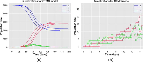
Figure 5. Five realizations generated by SSA for CTMC model (24(24) $\begin{array}{rl}P((S_{1,t+\mathrm{\Delta }t},I_{1,t+\mathrm{\Delta }})-(S_{1,t},I_{1,t})& =(-1,1))=S_{1,t}{\beta }_1[p_1{\displaystyle \frac{I_{1,t}}{N_1}}+p_2{\displaystyle \frac{I_{2,t}}{N_2}}]+o(\mathrm{\Delta }),\\ P((I_{1,t+\mathrm{\Delta }t},R_{1,t+\mathrm{\Delta }})-(I_{1,t},R_{1,t})& =(-1,1))=\gamma I_{1,t}+o(\delta ),\\ P((S_{2,t+\mathrm{\Delta }t},I_{2,t+\mathrm{\Delta }})-(S_{2,t},I_{2,t})& =(-1,1))=S_{2,t}{\beta }_2[p_1{\displaystyle \frac{I_{1,t}}{N_1}}+p_2{\displaystyle \frac{I_{2,t}}{N_2}}]+o(\mathrm{\Delta }),\\ P((I_{2,t+\mathrm{\Delta }t},R_{2,t+\mathrm{\Delta }})-(I_{2,t},R_{2,t})& =(-1,1))=\gamma I_{2,t}+o(\mathrm{\Delta })\end{array}$(24) ) with heterogeneous mixing. The top two subfigures are with initial condition of 1 infectious superspreader. The bottom two subfigures are with initial condition of 1 infectious non-superspreader.

Figure 6. The distribution of final epidemic sizes for ${10}^4$ realizations for CTMC model (21(21) $\begin{array}{rl}P((S_{t+\mathrm{\Delta }t},I_{t+\mathrm{\Delta }t},R_{t+\mathrm{\Delta }t})-(S_t,I_t,R_t)& =(-1,1,0))={\displaystyle \frac{\beta S_t{I}_t}{N}}\mathrm{\Delta }t+o(\mathrm{\Delta }t),\\ P((S_{t+\mathrm{\Delta }t},I_{t+\mathrm{\Delta }t},R_{t+\mathrm{\Delta }t})-(S_t,I_t,R_t)& =(0,-1,1))=\gamma I_t\mathrm{\Delta }t+o(\mathrm{\Delta }t),\end{array}$(21) ) with homogeneous mixing.

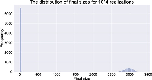
Figure 7. The distributions of final epidemic sizes for ${10}^4$ realizations for CTMC model (24(24) $\begin{array}{rl}P((S_{1,t+\mathrm{\Delta }t},I_{1,t+\mathrm{\Delta }})-(S_{1,t},I_{1,t})& =(-1,1))=S_{1,t}{\beta }_1[p_1{\displaystyle \frac{I_{1,t}}{N_1}}+p_2{\displaystyle \frac{I_{2,t}}{N_2}}]+o(\mathrm{\Delta }),\\ P((I_{1,t+\mathrm{\Delta }t},R_{1,t+\mathrm{\Delta }})-(I_{1,t},R_{1,t})& =(-1,1))=\gamma I_{1,t}+o(\delta ),\\ P((S_{2,t+\mathrm{\Delta }t},I_{2,t+\mathrm{\Delta }})-(S_{2,t},I_{2,t})& =(-1,1))=S_{2,t}{\beta }_2[p_1{\displaystyle \frac{I_{1,t}}{N_1}}+p_2{\displaystyle \frac{I_{2,t}}{N_2}}]+o(\mathrm{\Delta }),\\ P((I_{2,t+\mathrm{\Delta }t},R_{2,t+\mathrm{\Delta }})-(I_{2,t},R_{2,t})& =(-1,1))=\gamma I_{2,t}+o(\mathrm{\Delta })\end{array}$(24) ) with heterogeneous mixing, $(a)$ initiated by 1 infectious superspreader and $(b)$ initiated by 1 infectious non-superspreader.

Table 2. The probability of a minor outbreak for CTMC models (21(21) $\begin{array}{rl}P((S_{t+\mathrm{\Delta }t},I_{t+\mathrm{\Delta }t},R_{t+\mathrm{\Delta }t})-(S_t,I_t,R_t)& =(-1,1,0))={\displaystyle \frac{\beta S_t{I}_t}{N}}\mathrm{\Delta }t+o(\mathrm{\Delta }t),\\ P((S_{t+\mathrm{\Delta }t},I_{t+\mathrm{\Delta }t},R_{t+\mathrm{\Delta }t})-(S_t,I_t,R_t)& =(0,-1,1))=\gamma I_t\mathrm{\Delta }t+o(\mathrm{\Delta }t),\end{array}$(21) ) with initially 1 infectious individual, and (24(24) $\begin{array}{rl}P((S_{1,t+\mathrm{\Delta }t},I_{1,t+\mathrm{\Delta }})-(S_{1,t},I_{1,t})& =(-1,1))=S_{1,t}{\beta }_1[p_1{\displaystyle \frac{I_{1,t}}{N_1}}+p_2{\displaystyle \frac{I_{2,t}}{N_2}}]+o(\mathrm{\Delta }),\\ P((I_{1,t+\mathrm{\Delta }t},R_{1,t+\mathrm{\Delta }})-(I_{1,t},R_{1,t})& =(-1,1))=\gamma I_{1,t}+o(\delta ),\\ P((S_{2,t+\mathrm{\Delta }t},I_{2,t+\mathrm{\Delta }})-(S_{2,t},I_{2,t})& =(-1,1))=S_{2,t}{\beta }_2[p_1{\displaystyle \frac{I_{1,t}}{N_1}}+p_2{\displaystyle \frac{I_{2,t}}{N_2}}]+o(\mathrm{\Delta }),\\ P((I_{2,t+\mathrm{\Delta }t},R_{2,t+\mathrm{\Delta }})-(I_{2,t},R_{2,t})& =(-1,1))=\gamma I_{2,t}+o(\mathrm{\Delta })\end{array}$(24) ) with initially 1 infectious super-spreader and 1 infectious non super-spreader, respectively. It is demonstrated that, even with identical ${\mathcal{R}}_0$, the probability of a minor outbreak can be varied by different choice of epidemic models.

Summary of probabilities of a minor outbreak for CTMC models
Models (initial infection type)	BP estimates	SSA estimates
CTMC model (21(21) $\begin{array}{rl}P((S_{t+\mathrm{\Delta }t},I_{t+\mathrm{\Delta }t},R_{t+\mathrm{\Delta }t})-(S_t,I_t,R_t)& =(-1,1,0))={\displaystyle \frac{\beta S_t{I}_t}{N}}\mathrm{\Delta }t+o(\mathrm{\Delta }t),\\ P((S_{t+\mathrm{\Delta }t},I_{t+\mathrm{\Delta }t},R_{t+\mathrm{\Delta }t})-(S_t,I_t,R_t)& =(0,-1,1))=\gamma I_t\mathrm{\Delta }t+o(\mathrm{\Delta }t),\end{array}$(21) )	0.6602	0.6608
CTMC model (24(24) $\begin{array}{rl}P((S_{1,t+\mathrm{\Delta }t},I_{1,t+\mathrm{\Delta }})-(S_{1,t},I_{1,t})& =(-1,1))=S_{1,t}{\beta }_1[p_1{\displaystyle \frac{I_{1,t}}{N_1}}+p_2{\displaystyle \frac{I_{2,t}}{N_2}}]+o(\mathrm{\Delta }),\\ P((I_{1,t+\mathrm{\Delta }t},R_{1,t+\mathrm{\Delta }})-(I_{1,t},R_{1,t})& =(-1,1))=\gamma I_{1,t}+o(\delta ),\\ P((S_{2,t+\mathrm{\Delta }t},I_{2,t+\mathrm{\Delta }})-(S_{2,t},I_{2,t})& =(-1,1))=S_{2,t}{\beta }_2[p_1{\displaystyle \frac{I_{1,t}}{N_1}}+p_2{\displaystyle \frac{I_{2,t}}{N_2}}]+o(\mathrm{\Delta }),\\ P((I_{2,t+\mathrm{\Delta }t},R_{2,t+\mathrm{\Delta }})-(I_{2,t},R_{2,t})& =(-1,1))=\gamma I_{2,t}+o(\mathrm{\Delta })\end{array}$(24) ) (1 super-spreader)	0.6591	0.6660
CTMC model (24(24) $\begin{array}{rl}P((S_{1,t+\mathrm{\Delta }t},I_{1,t+\mathrm{\Delta }})-(S_{1,t},I_{1,t})& =(-1,1))=S_{1,t}{\beta }_1[p_1{\displaystyle \frac{I_{1,t}}{N_1}}+p_2{\displaystyle \frac{I_{2,t}}{N_2}}]+o(\mathrm{\Delta }),\\ P((I_{1,t+\mathrm{\Delta }t},R_{1,t+\mathrm{\Delta }})-(I_{1,t},R_{1,t})& =(-1,1))=\gamma I_{1,t}+o(\delta ),\\ P((S_{2,t+\mathrm{\Delta }t},I_{2,t+\mathrm{\Delta }})-(S_{2,t},I_{2,t})& =(-1,1))=S_{2,t}{\beta }_2[p_1{\displaystyle \frac{I_{1,t}}{N_1}}+p_2{\displaystyle \frac{I_{2,t}}{N_2}}]+o(\mathrm{\Delta }),\\ P((I_{2,t+\mathrm{\Delta }t},R_{2,t+\mathrm{\Delta }})-(I_{2,t},R_{2,t})& =(-1,1))=\gamma I_{2,t}+o(\mathrm{\Delta })\end{array}$(24) ) (1 non super-spreader)	0.9699	0.9683