Complexity of host-vector dynamics in a two-strain dengue model

Figures & data

Figure 1. Flow chart of the transitions between the host and vector compartments. The birth and death of hosts and vectors are not explicitly shown for the sake of clarity.

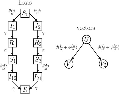
Figure 2. The range $(B_1,B_2)$ corresponding to 0, 1 or 2 coexistence equilibria (the dashed vertical line is the set with $B_1$ such that ${\mathcal{R}}_0=1$. The shaded area shows the pairs $(B_1,B_2)$ with a locally asymptotically stable interior equilibrium (eigenvalues computed numerically). The parameter values are given in Table 1 and $\varphi =0.5$.

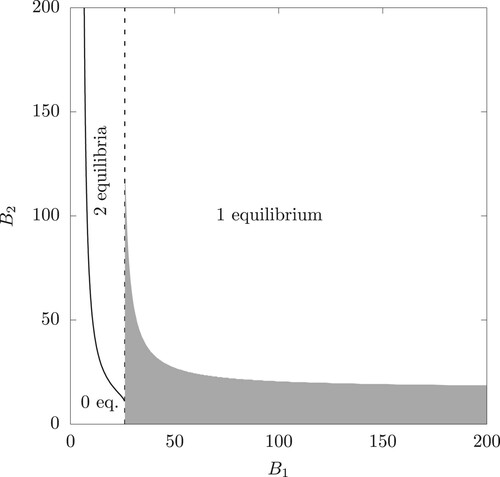
Table 1. Parameter values, most after [1,22] for the host-only model (A1) and [29] for the host-vector model.

Par.	Description
Host
N	Host population density	1000
$B_i$	Infection rate per infected vector	as indicated
${\beta }_i$	Infection rate per infected host	$[0,104]$ (or free)
μ	Susceptible birth rate	1/65
γ	Recovery rate	365/7
α	temporary cross-immunity rate	2, 52 or $[1,250]$
Vector
M	Vector population density	10000
ν	Susceptible birth rate	36.5
ϑ	Infection rate per host	73
η	Magnitude of sinusoidal fluctuation vectors	0 or 0.35
ϕ	Ratio of likelihoods of transmission from hosts with secondary and hosts with primary infection to vectors	$[0,12]$
φ	Phase	0

Notes: The units and values of the infection rate B in this study are different from those in the other references where it is β. Remark: in previous papers N was taken 100 but here 1000. This means that in the comparison the results for the compartments in the previous papers have to be corrected by multiplication with 10.

Table 2. List of bifurcation types.

Bifurcation	Description
H	Hopf bifurcation, real part of conjugate eigenvalues = 0
	equilibrium becomes unstable
	Origin of stable (supercritical $H^{-}$) or unstable (sub critical $H^{+}$) limit cycle
TC	Transcritical bifurcation
	Exchange of stability,
	One steady state enters the biologically relevant domain Ω
T	Tangent of limit cycle
	One Floquet multiplier = 1
	collision of two limit cycles
P	Pitchfork bifurcation of limit cycle
	One Floquet multiplier = 1
	Origin of two secondary stable limit cycle branches
GH	Bautin bifurcation, real part of conjugate eigenvalues = 0
	Origin of Tangent bifurcation T of limit cycle
TR	Torus bifurcation of limit cycle
	Pair of complex conjugate multipliers with magnitude = 1
	Origin of an invariant torus
C	Complex dynamics on a torus or chaos

Figure 3. Two-parameter $(\varphi ,\alpha )$ bifurcation diagram for the range $\varphi \in [0,12]$ and $\alpha \in [0,250]$. One Hopf bifurcation converges for $\alpha \to \mathrm{\infty }$ to the ϕ parameter value [†] for the model of [4] for (a) the host-only model (A1) from [1] and (b)  the host-vector model (1). [*] marks the value $\varphi =2.5$ in [18].

Figure 4. Two-parameter $(\varphi ,\alpha )$ bifurcation diagram for the range $\varphi \in [0,1.3]$ and $\alpha \in [1,7]$ (a) for the host-only model (A1) and (b) for the host-vector model (1).

Figure 5. One-parameter diagram for ϕ where $\alpha =2$ and B = 52. Equilibria or maximum and minimum values for limit cycles for total infected I (a) for the host-only model (A1) and (b) for the host-vector model (1). Red indicates stable and blue unstable solutions.

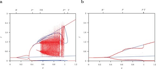
Figure 6. (a) Infected classes $I_1(t)$ (red), $I_2(t)$ (blue) unstable symmetric solutions for the limit cycle with parameter values $\alpha =2$, $\varphi =0.8$, B = 52 and normalized time for one period. (b) Infected classes $I_1^1(t_1)$ (red), $I_2^1(t_1)$ (blue) and $I_1^2(t_2)$ (green), $I_2^2(t_2)$ (pink) solutions for the two stable S-conjugate limit cycles.

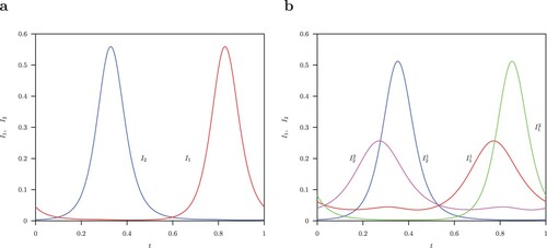
Figure 7. Two-parameter $(B,\vartheta )$ bifurcation diagram with parameter $\varphi =0.2$ of (a) the system (1), and (b) the QSSA system where the fast variables $V_1,V_2$ are assumed to be in steady state (9(9a) $\begin{array}{rl}{V}_1& =\frac{\vartheta M(I_1+\varphi I_{21})}{\vartheta (I_1+I_2+\varphi (I_{21}+I_{12}))+\nu N},\end{array}$(9a) ). TC curve is for values ${\mathcal{R}}_0=1$. Left of TC there is stable disease-free equilibrium where I = 0. Between the TC and H curve, there is a stable endemic equilibrium, and beyond H, there is a stable limit cycle. No pitchfork bifurcation P is observed in this parameter region.

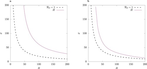
Figure 8. Two-parameter $(B,\vartheta )$ bifurcation diagram with parameter $\varphi =0.5$ of (a) the system (1), and (b) the QSSA system where the fast variables $V_1,V_2$ are assumed to be in steady state (9(9a) $\begin{array}{rl}{V}_1& =\frac{\vartheta M(I_1+\varphi I_{21})}{\vartheta (I_1+I_2+\varphi (I_{21}+I_{12}))+\nu N},\end{array}$(9a) ). TC curve is for values ${\mathcal{R}}_0=1$. Left of TC there is stable disease-free equilibrium where I = 0. Between the TC and H curve there is a stable endemic equilibrium, and between H and P, there is a stable limit cycle. Inside the region bordered by P, there is bistablity: a pair of S-symmetric limit cycles.

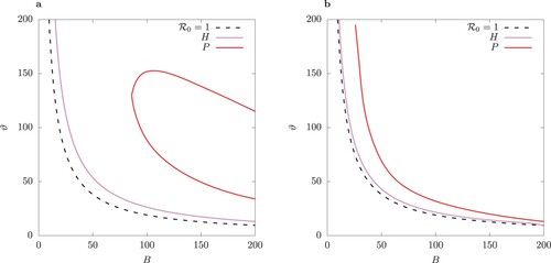
Figure 9. Two-parameter $(B,\vartheta )$ bifurcation diagram with parameter $\varphi =0.8$ of (a) the system (1), and (b) the QSSA system where the fast variables $V_1,V_2$ are assumed to be in steady state (9(9a) $\begin{array}{rl}{V}_1& =\frac{\vartheta M(I_1+\varphi I_{21})}{\vartheta (I_1+I_2+\varphi (I_{21}+I_{12}))+\nu N},\end{array}$(9a) ). TC curve is for values ${\mathcal{R}}_0=1$. Left of TC there is stable disease-free equilibrium where I = 0. Between the TC and H curve, there is a stable endemic equilibrium, and between H and P, there is a stable limit cycle. Inside the region bordered by P, there is bistablity: a pair of S-symmetric limit cycles.

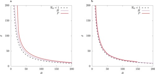
Figure 10. One-parameter bifurcation diagram for B for the case of equal infection rates $B_1=B_2=B$ in the host-vector model (1) (column (a)), and the QSSA model (column (b)). Solid lines indicate stable and dashed lines unstable solutions. Above the Hopf bifurcation point the minima and maxima for limit cycles are shown for total infected I for $\varphi =0.5$.

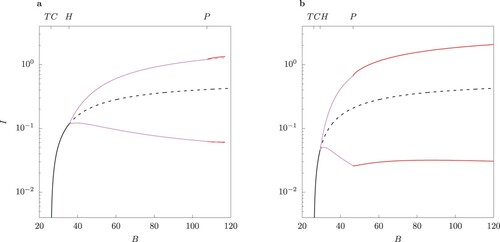
Figure 11. One-parameter bifurcation diagram for B for the case of equal infection rates $B_1=B_2=B$ in the host-vector model (1) (column (a)) and the QSSA model (column (b)). Solid lines indicate stable and dashed lines unstable solutions. Above the Hopf bifurcation point the minima and maxima for limit cycles are shown for total infected I for $\varphi =0.8$.

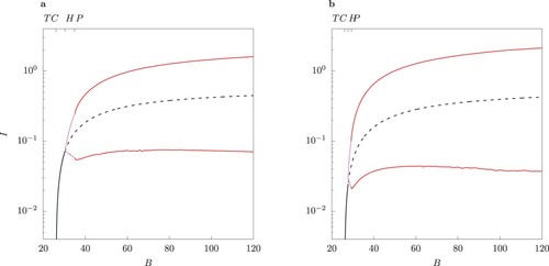
Figure 12. (a) One-parameter bifurcation diagram in B for the case $B_1=B_2=B$ when $\varphi =3$. Observe that in the range where two interior equilibria occur, both are locally asymptotically unstable. The dot ° marks the value of B where the two-strain equilibrium undergoes a subcritical Hopf bifurcation. (b) Phase portrait for B = 25.6 for two trajectories starting near the two unstable equilibria, marked by a dot °. The orange curve shows an epidemic with a single peak, later converging to extinction. Observe the oscillatory behaviour in the vicinity of the unstable limit cycle (red curve). c Phase portrait for B = 39.979. The trajectory follows an irregular regime.

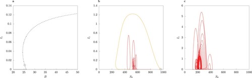
Figure 13. One-parameter diagram for ϕ where $\alpha =52$ and B = 52. Equilibria or maximum and minimum values for limit cycles for total infected I for (a) the host-only model [22] and (b) the host-vector model (1). Red indicates stable and blue unstable solutions.

Figure 14. Plot of the limit cycle trajectory. Colour coding: full model (red), QSSA model (blue), asymptotic expansion to second order in ε (black). Parameter values listed in Table 1 and (a) $B_{1,2}=50,\alpha =2,\varphi =0.5,\epsilon =0.1$, (b) $B_{1,2}=50,\alpha =2,\varphi =0.5,\epsilon =0.5$, and (c) $B_{1,2}=100,\alpha =2,\varphi =0.5,\epsilon =1$.

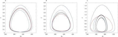
Figure 15. Two-strain non-autonomous host-vector model (1) and (3(3) $M=M(t)=M_0(1+\eta \cos \omega (t+\phi )).$(3) ) with B = 52. Torus bifurcation TR bifurcation exist at the same position as the Hopf H for the autonomous system (1), shown in Figure 3(b). L: limit cycle, C: complex dynamics. Details for the range $(\varphi ,\alpha )\in \{(0,1.3)\times (0,7)\}$ are shown enlarged in b.

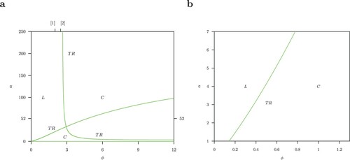
Figure 16. Two-strain non-autonomous (a) host-only model (A1) and (b) host-vector model (1) with parameter $\alpha =2$, with $\beta =104$ and $B=52$ respectively. For model (1) in forcing function (3) $M_0=10000$ and $\eta =0.1$ and in asimilar way for model (A1) in the forcing function in [2], Equation (2) ${\beta }_0=104$ and $\eta =0.5$. The bullets in (b) mark the globalmaximum and minimum values for limit cycles for total infected I. Red indicates stable and blue unstable solutions.

M. Aguiar, B.W. Kooi, and N. Stollenwerk, Epidemiology of dengue fever: a model with temporary cross-immunity and possible secondary infection shows bifurcations and chaotic behaviour in wide parameter regions, Math Model Nat. Phenom. 3 (2008), pp. 48–70.

 Web of Science ®Google Scholar

B.W. Kooi, M. Aguiar, and N. Stollenwerk, Bifurcation analysis of a family of multi-strain epidemiology models, J. Comput. Appl. Math. 252 (2013), pp. 148–158.

 Web of Science ®Google Scholar

F. Rocha, M. Aguiar, M. Souza, and N. Stollenwerk, Time-scale separation and centre manifold analysis describing vector-borne disease dynamics, Int. J. Comput. Math. 90(10) (2013), pp. 2105–2125.

 Web of Science ®Google Scholar

L. Billings, I.B. Schwartz, L.B. Shaw, M. McCrary, D.S. Burke, and D.A.T. Cummings, Instabilities in multiserotype disease models with antibody-dependent enhancement, J. Theor. Biol. 246 (2007), pp. 18–27.

 PubMed Web of Science ®Google Scholar

N. Ferguson, R. Anderson, and S. Gupta, The effect of antibody-dependent enhancement on the transmission dynamics and persistence of multiple-strain pathogens, Proc. Natl Acad. Sci. USA 96(9) (1999), pp. 790–794.

 PubMedGoogle Scholar

M. Aguiar, S. Ballesteros, B.W. Kooi, and N. Stollenwerk, The role of seasonality and import in a minimalistic multi-strain dengue model capturing differences between primary and secondary infections: complex dynamics and its implications for data analysis, J. Theor. Biol. 289 (2011), pp. 181–196.

 PubMed Web of Science ®Google Scholar