Building mean field ODE models using the generalized linear chain trick & Markov chain theory

Figures & data

Figure 1. Diagram for an SEIR-type model with an Erlang latent period and Coxian infectious period. A special case of Equations (15(15d) $\begin{array}{rl}\frac{\mathrm{d}R}{\mathrm{d}t}& =\overbrace{(-{\mathbf{A}}_{\mathbf{I}}\mathbf{1}{)}^{\mathsf{\text{T}}}\mathbf{y}}\end{array}$(15d) ) and Equations (20(20d) $\begin{array}{rl}\frac{\mathrm{d}R}{\mathrm{d}t}& =r_I{I}_{k_I}+\sum _{j=1}^{k_I-1}(1-{\rho }_{Ij}){\lambda }_{Ij}{I}_j.\end{array}$(20d) ). See the main text for details (and compare to Figure 2 in [83]).

Figure 2. SEIR-type model with heterogeneity in illness severity and hospitalizations that do not alter the infectious period. A special case of Equations (21(21e) $\begin{array}{rl}\frac{\mathrm{d}R}{\mathrm{d}t}& =(-{\mathbf{A}}_{{\mathbf{I}}_{\mathbf{0}}}\mathbf{1}{)}^{\mathsf{\text{T}}}{\mathbf{y}}_{\mathbf{0}}+(-{\mathbf{A}}_{{\mathbf{I}}_{\mathbf{s}}}\mathbf{1}{)}^{\mathsf{\text{T}}}{\mathbf{y}}_{\mathbf{s}}.\end{array}$(21e) ) (cf. Figure 3). See the main text for details. Here the standard LCT has been applied to the exposed (E) state, and the GLCT is applied to the I states, using the competing Poisson process approach [51] to model hospitalizations in a fraction of the I state individuals. This ensures that the time spent in I is independent of whether or not individuals transition to the hospital or not. Compare to [35].

Figure 3. SEIR-type model with heterogeneity in illness severity in which a fraction of infected individuals experience severe illness, and a fraction of those require critical care. This is also a special case of Equations (21(21e) $\begin{array}{rl}\frac{\mathrm{d}R}{\mathrm{d}t}& =(-{\mathbf{A}}_{{\mathbf{I}}_{\mathbf{0}}}\mathbf{1}{)}^{\mathsf{\text{T}}}{\mathbf{y}}_{\mathbf{0}}+(-{\mathbf{A}}_{{\mathbf{I}}_{\mathbf{s}}}\mathbf{1}{)}^{\mathsf{\text{T}}}{\mathbf{y}}_{\mathbf{s}}.\end{array}$(21e) ) (see Figure 2). See the main text for details.

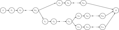
Figure 4. Benchmark results for 140 iterations computing numerical solutions to Rosenzweig-MacArthur model with Erlang (gamma) distributed maturation times and time spent in the adult-stage, using either a direct (LCT; medium grey) or more general (GLCT; black) formulations of the model (the standard Rosenzweig-MacArthur model with no maturation delay and exponentially distributed time spent in the adult stage [light grey; Equations (8(8b) $\begin{array}{rl}\frac{\mathrm{d}P}{\mathrm{d}t}& =\chi \frac{aN}{h+N}P-\mu P\end{array}$(8b) )] is also included as a baseline). The second and third cases are mathematically equivalent systems. For smaller shape parameters (lower dimension systems) the GLCT model formulation is relatively slower than explicitly writing out the 2M + 1 equations, whereas for larger shape parameters (higher dimension systems) the GLCT-based formulation becomes markedly faster. This is likely due to the efficiency of the matrix computations. The x-axis values M indicate the number of maturing predator sub-states ($k_x=M$) and adult predator sub-states ($k_y=M$), which yields a 2M + 1 dimensional model. Numerical solutions were computed using the ode() function in the deSolve package [101] in R [90], using method ode45 with atol=10-6, for time points 0 to 500 in increments of 1, and model parameters r = 1, K = 1000, a = 5, h = 500, $\chi =0.5$, ${\mu }_x=0.5$, ${\mu }_y=1$, with initial conditions $N(0)=1000$, $x_i(0)=0$ ($i\ge 1$), $y_1(0)=10$, and $y_j(0)=0$ (j>1).

Figure 5. Benchmark results for 500 iterations computing numerical solutions to an SEIR model with latent and infectious period distributions that are either Erlang (panel a; Equation (18(18d) $\begin{array}{rl}\frac{\mathrm{d}R}{\mathrm{d}t}& =\frac{k_I}{{\tau }_I}{I}_{k_I}\end{array}$(18d) )) or Coxian (panel b; Equation (20(20d) $\begin{array}{rl}\frac{\mathrm{d}R}{\mathrm{d}t}& =r_I{I}_{k_I}+\sum _{j=1}^{k_I-1}(1-{\rho }_{Ij}){\lambda }_{Ij}{I}_j.\end{array}$(20d) )), using either a direct equation-by-equation formulation (LCT; medium grey) or more general matrix-vector formulation (GLCT; black) of the model (SEIR with exponentially distributed latent and infectious periods [light grey; Equation (14)] also included as a baseline). The second and third cases are mathematically equivalent systems. For smaller shape parameters (lower dimension systems) the GLCT model formulation is relatively slower than explicitly writing out the 2N + 2 equations, whereas for larger shape parameters (higher dimension systems) the GLCT-based formulation becomes faster, presumably due to the efficiency of the matrix computations. The x-axis values N indicate the number of sub-states in each of E ($k_E=N$) and I ($k_I=N$), which yields a 2N + 2 dimensional model. Numerical solutions were computed using the ode() function in the deSolve package [101] in R [90], using method ode45 with atol=10-6, for time points 0 to 100 in increments of 0.5, and model parameters $\beta =1$, ${\mu }_E=4$, ${\mu }_I=7$, where all ${\rho }_E={\rho }_I=0.99$, with initial conditions $S(0)=0.9999$, $E_1(0)=0.0001$, $E_i(0)=0$ (i>1), $I_1(0)=0$, $I_i(0)=0$ (i>1), and $R(0)=0$. See Supplementary Materials for more details.

A. Nande, B. Adlam, J. Sheen, M.Z. Levy, and A.L. Hill, Dynamics of COVID-19 under social distancing measures are driven by transmission network structure, PLOS Comput. Biol. 17 (2021), p. e1008684.

 PubMed Web of Science ®Google Scholar

P.J. Hurtado and A.S. Kirosingh, Generalizations of the ‘linear chain trick’: incorporating more flexible dwell time distributions into mean field ODE models, J. Math. Bio. 79 (2019), pp. 1831–1883.

 PubMed Web of Science ®Google Scholar

Z. Feng, Y. Zheng, N. Hernandez-Ceron, H. Zhao, J.W. Glasser, and A.N. Hill, Mathematical models of Ebola-Consequences of underlying assumptions, Math. Biosci. 277 (2016), pp. 89–107.

 PubMed Web of Science ®Google Scholar

K. Soetaert, T. Petzoldt, and R.W. Setzer, Solving differential equations in R: package deSolve, J. Stat. Softw. 33 (2010), pp. 1–25Available at http://www.jstatsoft.org/v33/i09

 PubMed Web of Science ®Google Scholar

R Core Team, A Language and Environment for Statistical Computing, R Foundation for Statistical Computing, Vienna, Austria , 2020. Available at https://www.R-project.org/.

 Google Scholar