Delay in budget allocation for vaccination and awareness induces chaos in an infectious disease model

Figures & data

Figure 1. Schematic diagram for systems (1(1) $\begin{array}{rl}\frac{\mathrm{d}S}{\mathrm{d}t}& =\mathrm{\Lambda }-\left(\text{β}-{\text{β}}_1\frac{k_{1}M}{p+k_{1}M}\right)SI-\varphi \frac{(1-k_1)M}{q+(1-k_1)M}S+\nu I+\delta V-\mathrm{d}S,\\ \frac{\mathrm{d}I}{\mathrm{d}t}& =\left(\text{β}-{\text{β}}_1\frac{k_{1}M}{p+k_{1}M}\right)SI-(\nu +\alpha +d)I,\\ \frac{\mathrm{d}V}{\mathrm{d}t}& =\varphi \frac{(1-k_1)M}{q+(1-k_1)M}S-(\delta +d)V,\\ \frac{\mathrm{d}M}{\mathrm{d}t}& =rM\left(1-\frac{M}{K}\right)+\theta IM.\end{array}$(1) ) and (16(16) $\begin{array}{rl}\frac{\mathrm{d}I}{\mathrm{d}t}& =\left(\text{β}-{\text{β}}_1\frac{k_{1}M}{p+k_{1}M}\right)(N-I-V)I-(\nu +\alpha +d)I,\\ \frac{\mathrm{d}V}{\mathrm{d}t}& =\frac{\varphi (1-k_1)M}{q+(1-k_1)M}(N-I-V)-(\delta +d)V,\\ \frac{\mathrm{d}N}{\mathrm{d}t}& =\mathrm{\Lambda }-\mathrm{d}N-\alpha I,\\ \frac{\mathrm{d}M}{\mathrm{d}t}& =rM\left(1-\frac{M}{K}\right)+\theta I(t-\tau )M.\end{array}$(16) ). Here, red colour denotes the impact of budget allocation in reducing the transmission rate by making people aware about the disease whereas blue colour stands for the utilization of budget on vaccinating the susceptible individuals; time delay involved in per-capita growth rate of budget allocation due to increase in infected individuals is represented by cyan colour.

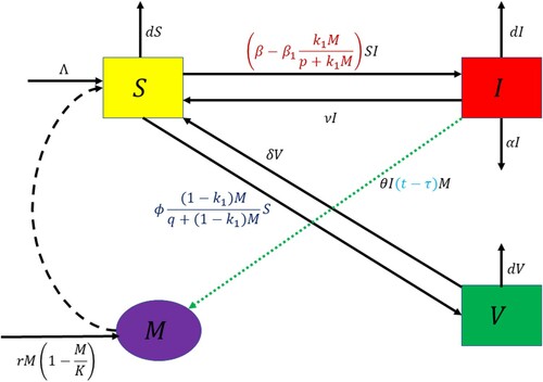
Table 1. Descriptions of parameters involved in system (1(1) $\begin{array}{rl}\frac{\mathrm{d}S}{\mathrm{d}t}& =\mathrm{\Lambda }-\left(\text{β}-{\text{β}}_1\frac{k_{1}M}{p+k_{1}M}\right)SI-\varphi \frac{(1-k_1)M}{q+(1-k_1)M}S+\nu I+\delta V-\mathrm{d}S,\\ \frac{\mathrm{d}I}{\mathrm{d}t}& =\left(\text{β}-{\text{β}}_1\frac{k_{1}M}{p+k_{1}M}\right)SI-(\nu +\alpha +d)I,\\ \frac{\mathrm{d}V}{\mathrm{d}t}& =\varphi \frac{(1-k_1)M}{q+(1-k_1)M}S-(\delta +d)V,\\ \frac{\mathrm{d}M}{\mathrm{d}t}& =rM\left(1-\frac{M}{K}\right)+\theta IM.\end{array}$(1) ).

Parameters	Descriptions	Units	Values	Sources
Λ	Immigration into the class of susceptible	person day${}^{-1}$	2	Assumed
	population
β	Contact rate of susceptible with	person${}^{-1}$day${}^{-1}$	0.000024	Assumed
	infected individuals in absence of funds
${\text{β}}_1$	Efficacy of budget allocation to reduce	person${}^{-1}$day${}^{-1}$	0.000012	[35]
	the contact rate via propagating awareness
$k_1$	Fraction of budget allocated to	–	0.4	Assumed
	warn susceptibles via propagating awareness
p	Half saturation constant	dollar	50	Assumed
ϕ	Vaccination rate among susceptible individuals	day${}^{-1}$	0.004	Assumed
	in the presence of budget allocation
q	Half saturation constant	dollar	150	Assumed
δ	Rate of transfer of vaccinated individuals to	day${}^{-1}$	0.003	Assumed
	susceptible class due to ineffectiveness of vaccine
ν	Recovery rate of human population	day${}^{-1}$	0.34	[29]
α	Disease-induced death rate of human population	day${}^{-1}$	0.0002	Assumed
d	Natural death rate of human population	day${}^{-1}$	0.00004	[17]
r	Intrinsic growth rate of budget allocation	day${}^{-1}$	0.5	Assumed
K	Carrying capacity of budget allocation	dollar	500	Assumed
θ	Per-capita growth rate of budget allocation due	person${}^{-1}$day${}^{-1}$	0.0005	Assumed
	to increase in infected individuals

Figure 2. Normalized forward sensitivity indices of (a) ${\mathcal{R}}_{\mathrm{a}\mathrm{v}}$, (b) ${\text{β}}_{1_c}$ and (c) ${\varphi }_c$ with respect to model parameters. Parameters are at the same values as in Table 1 except $\alpha =0.02$.

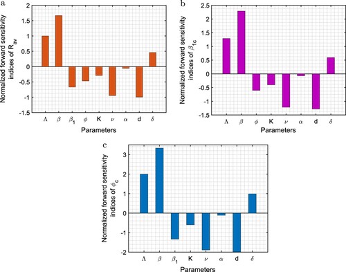
Figure 3. Semi-relative sensitivity solutions for infective population (I) and budget allocation (M) with respect to the parameters β, ${\text{β}}_1$, ϕ and θ. Parameters are at the same values as in Table 1.

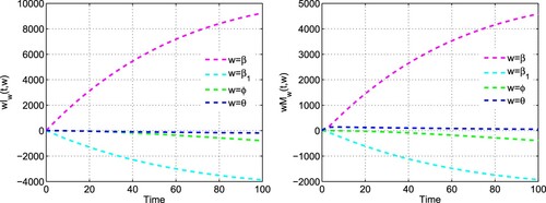
Figure 4. Contour plots of the basic reproduction number (${\mathcal{R}}_{\mathrm{a}\mathrm{v}}$) with respect to (a) ${\text{β}}_1$ and K, and (b) ϕ and K. The dashed blue line represents ${\mathcal{R}}_{\mathrm{a}\mathrm{v}}=1$. Rest of the parameters are at the same values as in Table 1.

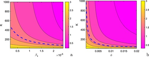
Figure 5. Contour plots of (a) ${\text{β}}_{1_c}$ with respect to ϕ and δ, and (b) ${\varphi }_c$ with respect to ${\text{β}}_1$ and δ. Rest of the parameters are at the same values as in Table 1.

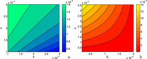
Figure 6. Surface plots of infective population (I) with respect to (a) ${\text{β}}_1$ and p, (b) ϕ and q, (c) K and δ, and (d) θ and δ. Rest of the parameters are at the same values as in Table 1.

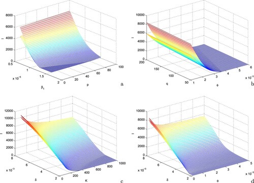
Figure 7. Effects of vaccination and awareness on the equilibrium level of infective population. Parameters are at the same values as in Table 1.

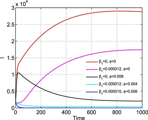
Figure 8. Variation of infected population $I\left(t\right)$ with respect to time t for different values of $k_1$: (a) for ${\mathcal{H}}_1>{\mathcal{H}}_2$ i.e. $k_1<k_{1_c}=0.4393$ and (b) for ${\mathcal{H}}_1<{\mathcal{H}}_2$ i.e. $k_1>k_{1_c}$. Rest of the parameters are at the same values as in Table 1.

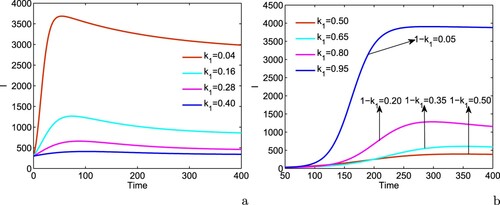
Figure 9. Forward bifurcation diagram of system (2(2) $\begin{array}{rl}\frac{\mathrm{d}I}{\mathrm{d}t}& =\left(\text{β}-{\text{β}}_1\frac{k_{1}M}{p+k_{1}M}\right)(N-I-V)I-(\nu +\alpha +d)I,\\ \frac{\mathrm{d}V}{\mathrm{d}t}& =\varphi \frac{(1-k_1)M}{q+(1-k_1)M}(N-I-V)-(\delta +d)V,\\ \frac{\mathrm{d}N}{\mathrm{d}t}& =\mathrm{\Lambda }-\mathrm{d}N-\alpha I,\\ \frac{\mathrm{d}M}{\mathrm{d}t}& =rM\left(1-\frac{M}{K}\right)+\theta IM.\end{array}$(2) ). Parameters are at the same values as in Table 1. Blue colour denotes stable disease-free equilibrium ($E_3$), red colour represents unstable disease-free equilibrium ($E_3$) and magenta colour stands for stable interior equilibrium ($E^{\ast }$).

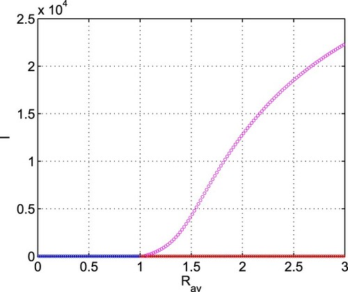
Figure 10. Global stability of the equilibrium $E^{\ast }$ in I−V −M space. Parameters are at the same values as in Table 1.

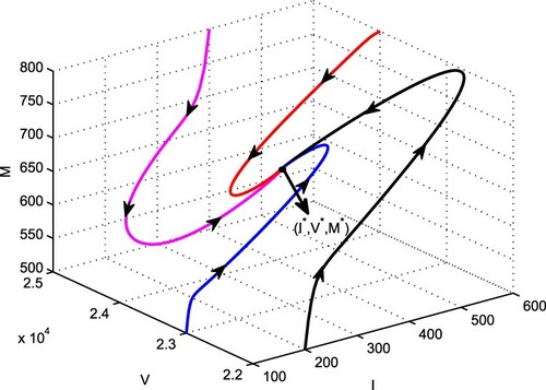
Figure 11. Bifurcation diagram of system (1(1) $\begin{array}{rl}\frac{\mathrm{d}S}{\mathrm{d}t}& =\mathrm{\Lambda }-\left(\text{β}-{\text{β}}_1\frac{k_{1}M}{p+k_{1}M}\right)SI-\varphi \frac{(1-k_1)M}{q+(1-k_1)M}S+\nu I+\delta V-\mathrm{d}S,\\ \frac{\mathrm{d}I}{\mathrm{d}t}& =\left(\text{β}-{\text{β}}_1\frac{k_{1}M}{p+k_{1}M}\right)SI-(\nu +\alpha +d)I,\\ \frac{\mathrm{d}V}{\mathrm{d}t}& =\varphi \frac{(1-k_1)M}{q+(1-k_1)M}S-(\delta +d)V,\\ \frac{\mathrm{d}M}{\mathrm{d}t}& =rM\left(1-\frac{M}{K}\right)+\theta IM.\end{array}$(1) ) with respect to θ. Rest of the parameters are at the same values as in (24(24) $\begin{array}{rl}& \mathrm{\Lambda }=5,\text{β}=0.0000030,{\text{β}}_1=0.0000018,k_1=0.2,p=2000,\varphi =0.02,q=2500,\\ & \delta =0.008,\nu =0.22,\alpha =0.00001,d=0.00004,r=0.006,K=500.\end{array}$(24) ). Here, red colour represents the upper limit of oscillation cycle and blue colour represents the lower limit of oscillation cycle.

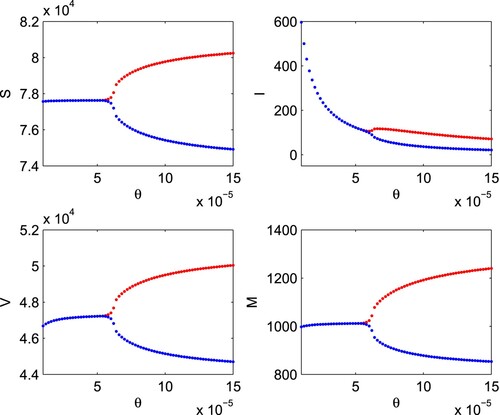
Figure 12. Bifurcation diagram of system (16(16) $\begin{array}{rl}\frac{\mathrm{d}I}{\mathrm{d}t}& =\left(\text{β}-{\text{β}}_1\frac{k_{1}M}{p+k_{1}M}\right)(N-I-V)I-(\nu +\alpha +d)I,\\ \frac{\mathrm{d}V}{\mathrm{d}t}& =\frac{\varphi (1-k_1)M}{q+(1-k_1)M}(N-I-V)-(\delta +d)V,\\ \frac{\mathrm{d}N}{\mathrm{d}t}& =\mathrm{\Lambda }-\mathrm{d}N-\alpha I,\\ \frac{\mathrm{d}M}{\mathrm{d}t}& =rM\left(1-\frac{M}{K}\right)+\theta I(t-\tau )M.\end{array}$(16) ) with respect to τ. Rest of the parameters are at the same values as in (25(25) $\begin{array}{rl}& \mathrm{\Lambda }=400,\text{β}=0.000048,{\text{β}}_1=0.000040,k_1=0.4,p=60,\varphi =0.005,q=120,\\ & \delta =0.008,\nu =0.3,\alpha =0.02,d=0.01,r=0.005,K=500,\theta =\mathrm{0.00005.}\end{array}$(25) ). Here, blue colour represents stability of the interior equilibrium and magenta colour corresponds to instability of the interior equilibrium.

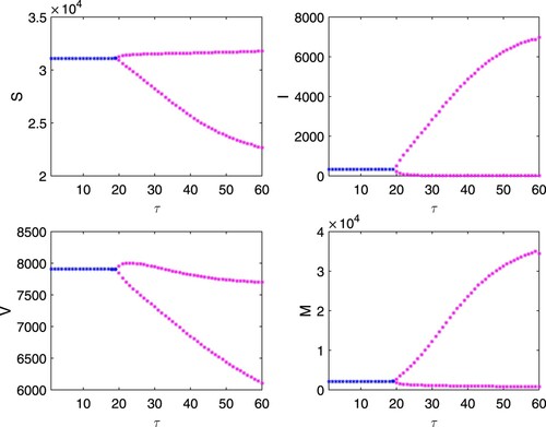
Table 2. Critical values of τ.

${\tau }_0^{+}$=61 days	${\tau }_1^{+}$=225 days	${\tau }_2^{+}$=390 days	${\tau }_3^{+}$=554 days	···
${\tau }_0^{-}$=156 days	${\tau }_1^{-}$=472 days	${\tau }_2^{-}$=788 days	${\tau }_3^{-}$=1105 days	···

Figure 13. Time series of system (16(16) $\begin{array}{rl}\frac{\mathrm{d}I}{\mathrm{d}t}& =\left(\text{β}-{\text{β}}_1\frac{k_{1}M}{p+k_{1}M}\right)(N-I-V)I-(\nu +\alpha +d)I,\\ \frac{\mathrm{d}V}{\mathrm{d}t}& =\frac{\varphi (1-k_1)M}{q+(1-k_1)M}(N-I-V)-(\delta +d)V,\\ \frac{\mathrm{d}N}{\mathrm{d}t}& =\mathrm{\Lambda }-\mathrm{d}N-\alpha I,\\ \frac{\mathrm{d}M}{\mathrm{d}t}& =rM\left(1-\frac{M}{K}\right)+\theta I(t-\tau )M.\end{array}$(16) ) for different values of τ. Systems shows (a) stable focus at $\tau =30$, (b) limit cycle oscillations at $\tau =100$, (c) stable focus at $\tau =180$ and (d) chaotic dynamics at $\tau =400$. Rest of the parameters are at the same values as in (25(25) $\begin{array}{rl}& \mathrm{\Lambda }=400,\text{β}=0.000048,{\text{β}}_1=0.000040,k_1=0.4,p=60,\varphi =0.005,q=120,\\ & \delta =0.008,\nu =0.3,\alpha =0.02,d=0.01,r=0.005,K=500,\theta =\mathrm{0.00005.}\end{array}$(25) ) except ${\text{β}}_1=0.000034$, p = 500, q = 800, $\varphi =0.05$, $\delta =0.08$.

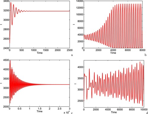
Figure 14. Bifurcation diagram of system (16(16) $\begin{array}{rl}\frac{\mathrm{d}I}{\mathrm{d}t}& =\left(\text{β}-{\text{β}}_1\frac{k_{1}M}{p+k_{1}M}\right)(N-I-V)I-(\nu +\alpha +d)I,\\ \frac{\mathrm{d}V}{\mathrm{d}t}& =\frac{\varphi (1-k_1)M}{q+(1-k_1)M}(N-I-V)-(\delta +d)V,\\ \frac{\mathrm{d}N}{\mathrm{d}t}& =\mathrm{\Lambda }-\mathrm{d}N-\alpha I,\\ \frac{\mathrm{d}M}{\mathrm{d}t}& =rM\left(1-\frac{M}{K}\right)+\theta I(t-\tau )M.\end{array}$(16) ) with respect to τ. Rest of the parameters are at the same values as in (25(25) $\begin{array}{rl}& \mathrm{\Lambda }=400,\text{β}=0.000048,{\text{β}}_1=0.000040,k_1=0.4,p=60,\varphi =0.005,q=120,\\ & \delta =0.008,\nu =0.3,\alpha =0.02,d=0.01,r=0.005,K=500,\theta =\mathrm{0.00005.}\end{array}$(25) ) except ${\text{β}}_1=0.000034$, p = 500, q = 800, $\varphi =0.05$, $\delta =0.08$. Here, red colour represents the upper limit of oscillation cycle and blue colour represents the lower limit of oscillation cycle.

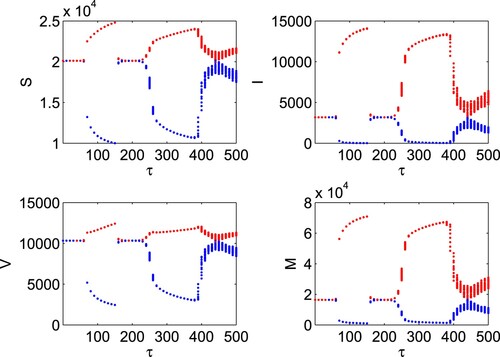
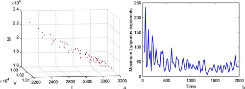
Figure 15. (a) Poincaré map of the system (16(16) $\begin{array}{rl}\frac{\mathrm{d}I}{\mathrm{d}t}& =\left(\text{β}-{\text{β}}_1\frac{k_{1}M}{p+k_{1}M}\right)(N-I-V)I-(\nu +\alpha +d)I,\\ \frac{\mathrm{d}V}{\mathrm{d}t}& =\frac{\varphi (1-k_1)M}{q+(1-k_1)M}(N-I-V)-(\delta +d)V,\\ \frac{\mathrm{d}N}{\mathrm{d}t}& =\mathrm{\Lambda }-\mathrm{d}N-\alpha I,\\ \frac{\mathrm{d}M}{\mathrm{d}t}& =rM\left(1-\frac{M}{K}\right)+\theta I(t-\tau )M.\end{array}$(16) ) in I−V −M space at S = 20000 for $\tau =4000$ days, and (b) maximum Lyapunov exponent of the system (16(16) $\begin{array}{rl}\frac{\mathrm{d}I}{\mathrm{d}t}& =\left(\text{β}-{\text{β}}_1\frac{k_{1}M}{p+k_{1}M}\right)(N-I-V)I-(\nu +\alpha +d)I,\\ \frac{\mathrm{d}V}{\mathrm{d}t}& =\frac{\varphi (1-k_1)M}{q+(1-k_1)M}(N-I-V)-(\delta +d)V,\\ \frac{\mathrm{d}N}{\mathrm{d}t}& =\mathrm{\Lambda }-\mathrm{d}N-\alpha I,\\ \frac{\mathrm{d}M}{\mathrm{d}t}& =rM\left(1-\frac{M}{K}\right)+\theta I(t-\tau )M.\end{array}$(16) ) at $\tau =400$ days. Rest of the parameters are at the same values as in (25(25) $\begin{array}{rl}& \mathrm{\Lambda }=400,\text{β}=0.000048,{\text{β}}_1=0.000040,k_1=0.4,p=60,\varphi =0.005,q=120,\\ & \delta =0.008,\nu =0.3,\alpha =0.02,d=0.01,r=0.005,K=500,\theta =\mathrm{0.00005.}\end{array}$(25) ) except ${\text{β}}_1=0.000034$, p = 500, q = 800, $\varphi =0.05$, $\delta =0.08$.

A.K. Misra, R.K. Rai, and Y. Takeuchi, Modeling the effect of time delay in budget allocation to control an epidemic through awareness, Int. J. Biomath. 11(2) (2018), pp. 1850027(1–20).

 Web of Science ®Google Scholar

S. Lee, G. Chowell, and C. Castillo-Chavez, Optimal control for pandemic influenza: The role of limited antiviral treatment and isolation, J. Theor. Biol. 265 (2010), pp. 136–150.

 PubMed Web of Science ®Google Scholar

H. Gaff and E. Schaefer, Optimal control applied to vaccination and treatment strategies for various epidemiological models, Math. Biosci. Eng. 6(3) (2009), pp. 469–492.

 PubMed Web of Science ®Google Scholar