Discrete dynamical models on Wolbachia infection frequency in mosquito populations with biased release ratios

Figures & data

Figure 1. The division of the $\mu \alpha$-plane depending on the signs of $D(\mu ,\alpha )$, $f(0,\alpha )$ and ${\mathrm{\Gamma }}_x\left(\alpha \right)$. It shows that the curves ${\alpha }_1^{\ast }\left(\mu \right)$, ${\alpha }_2^{\ast }\left(\mu \right)$ and ${\alpha }_3^{\ast }$ divide the $\mu \alpha$-plane into six subregions: ${\mathrm{\Omega }}_1=\left\{\right(\mu ,\alpha ):D(\mu ,\alpha )>0,f(0,\alpha )>0,{\mathrm{\Gamma }}_x(\alpha )>0\}$, ${\mathrm{\Omega }}_2=\left\{\right(\mu ,\alpha ):D(\mu ,\alpha )>0,f(0,\alpha )<0,{\mathrm{\Gamma }}_x(\alpha )>0\}$, ${\mathrm{\Omega }}_3=\left\{\right(\mu ,\alpha ):D(\mu ,\alpha )>0,f(0,\alpha )<0,{\mathrm{\Gamma }}_x(\alpha )<0\}$, ${\mathrm{\Omega }}_4=\left\{\right(\mu ,\alpha ):D(\mu ,\alpha )>0,f(0,\alpha )>0,{\mathrm{\Gamma }}_x(\alpha )<0\}$, ${\mathrm{\Omega }}_5=\left\{\right(\mu ,\alpha ):D(\mu ,\alpha )<0,f(0,\alpha )>0,{\mathrm{\Gamma }}_x(\alpha )<0\}$ and ${\mathrm{\Omega }}_6=\left\{\right(\mu ,\alpha ):D(\mu ,\alpha )<0,f(0,\alpha )>0,{\mathrm{\Gamma }}_x(\alpha )>0\}$. There exist two positive equilibria in subregion ${\mathrm{\Omega }}_1$ (yellow), a unique positive equilibrium in subregions ${\mathrm{\Omega }}_2\cup {\mathrm{\Omega }}_3$ and two curves $\alpha ={\alpha }_2^{\ast }\left(\mu \right)$ for $\mu \in (0,{\mu }_2^{\ast }/2)$, and $\alpha ={\alpha }_1^{\ast }\left(\mu \right)$ for $\mu \in ({\mu }_1^{\ast },{\mu }_2^{\ast }/2)$ (red), and no positive equilibria in subregions ${\mathrm{\Omega }}_4\cup {\mathrm{\Omega }}_5\cup {\mathrm{\Omega }}_6$ together with the curve $\alpha ={\alpha }_2^{\ast }\left(\mu \right)$ for $\mu \in [{\mu }_2^{\ast }/2,{\mu }_2^{\ast })$ (blue).

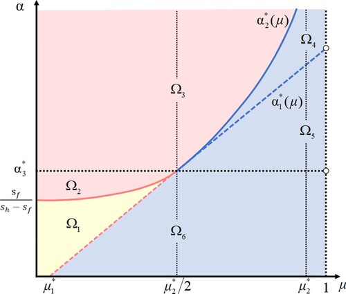
Figure 2. Given $s_f=0.1$ and $s_h=0.9$, we have ${\mu }_1^{\ast }\approx 0.1975$. For the case $\mu =0.15<{\mu }_1^{\ast }$, we get $x_1^{\ast }\left(\mu \right)\approx 0.3375$, $x_2^{\ast }\left(\mu \right)\approx 0.7736$. Numerical trials imply that ${\text{β}}_1^{\ast }\approx 0.0255$. Taking $\text{β}=0.01<{\text{β}}_1^{\ast }$, we have $x_1^{\ast }(\mu ,\text{β})\approx 0.0367$, $x_2^{\ast }(\mu ,\text{β})\approx 0.2987$ and $x_3^{\ast }(\mu ,\text{β})\approx 0.7758$. At ${\text{β}}_1^{\ast }$, $x_1^{\ast }(\mu ,{\text{β}}_1^{\ast })=x_2^{\ast }(\mu ,{\text{β}}_1^{\ast })\approx 0.1661$ and $x_3^{\ast }(\mu ,{\text{β}}_1^{\ast })\approx 0.7788$. Furthermore, when increasing β to 0.004, both $x_1^{\ast }(\mu ,\text{β})$ and $x_2^{\ast }(\mu ,\text{β})$ vanish, and $x_3^{\ast }(\mu ,\text{β})\approx 0.7815$.

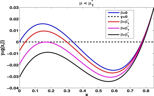
Figure 3. Given $s_f=0.1$ and $s_h=0.9$, we take $\mu ={\mu }_1^{\ast }\approx 0.1975$. When $\text{β}=0$, $x_1^{\ast }\left({\mu }_1^{\ast }\right)$ and $x_2^{\ast }\left({\mu }_1^{\ast }\right)$ coincide to $x_1^{\ast }\left({\mu }_1^{\ast }\right)=x_2^{\ast }\left({\mu }_1^{\ast }\right)\approx 0.5556$. Numerical trials offer ${\text{β}}_2^{\ast }\approx 0.0426$. When $\text{β}=0.02<{\text{β}}_2^{\ast }$, $x_1^{\ast }({\mu }_1^{\ast },\text{β})\approx 0.0606$, $x_2^{\ast }({\mu }_1^{\ast },\text{β})\approx 0.4209$ and $x_3^{\ast }({\mu }_1^{\ast },\text{β})\approx 0.6296$. When $\text{β}={\text{β}}_2^{\ast }$, both $x_1^{\ast }({\mu }_1^{\ast },{\text{β}}_2^{\ast })$ and $x_2^{\ast }({\mu }_1^{\ast },{\text{β}}_2^{\ast })$ coincide to $x_1^{\ast }({\mu }_1^{\ast },{\text{β}}_2^{\ast })=x_2^{\ast }({\mu }_1^{\ast },{\text{β}}_2^{\ast })\approx 0.2280$ and $x_3^{\ast }({\mu }_1^{\ast },{\text{β}}_2^{\ast })\approx 0.6539$. For $\text{β}=0.08>{\text{β}}_2^{\ast }$, $x_3^{\ast }({\mu }_1^{\ast },\text{β})\approx 0.6772$.

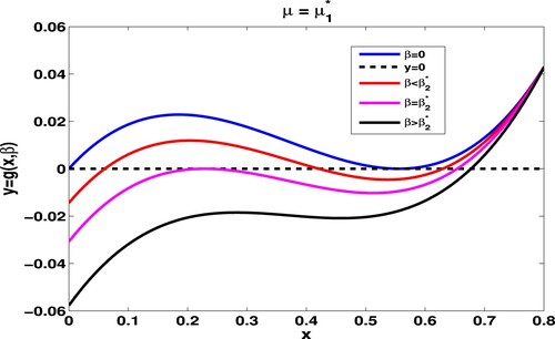
Figure 4. Given $s_f=0.1$ and $s_h=0.9$, we take $\mu =0.2>{\mu }_1^{\ast }\approx 0.1975$. Numerical simulations show that ${\text{β}}_3^{\ast }\approx 0.0057$, ${\text{β}}_4^{\ast }\approx 0.0437$. The number of zeros of $g(x,\text{β})$ lying in $(0,1)$ goes from 1, passing 2, 3, 2, and finally to 1 as β increases from 0 to the β with $\text{β}>{\text{β}}_4^{\ast }$.

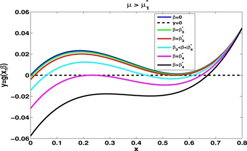
Figure 5. Distable dynamics driven by model (4(4) $x_{n+1}=\frac{(1-\mu )(1-s_f)(1+\alpha )x_n}{s_h{x}_n^2-[s_f+s_h+\alpha (s_f-s_h\left)\right]x_n+1+\alpha (1-s_h)},n=0,1,2,\dots .$(4) ) and model (16(16) $x_{n+1}=\frac{(1-\mu )(1-s_f)(\text{β}+x_n)}{s_h{x}_n^2-(s_f+s_h)x_n+1+\text{β}(1-s_f)},n=0,1,2,\dots .$(16) ). Panel (A) is for model (4(4) $x_{n+1}=\frac{(1-\mu )(1-s_f)(1+\alpha )x_n}{s_h{x}_n^2-[s_f+s_h+\alpha (s_f-s_h\left)\right]x_n+1+\alpha (1-s_h)},n=0,1,2,\dots .$(4) ) and Panel (B) is for model (16(16) $x_{n+1}=\frac{(1-\mu )(1-s_f)(\text{β}+x_n)}{s_h{x}_n^2-(s_f+s_h)x_n+1+\text{β}(1-s_f)},n=0,1,2,\dots .$(16) ).

Figure 6. Comparisons on the infection frequency thresholds (A) and the polymorphic states (B) driven by (3(3) $\begin{array}{rl}{x}_{n+1}& =\frac{(1-\mu )(1-s_f)(1+r)(x_n+r)}{s_h{x}_n^2-\left[s_f+s_h+r(s_f-s_h)\right]x_n+1+(2-s_f-s_h)r+(1-s_f)r^2},\\ & n=0,1,2,\dots \end{array}$(3) ), (16(16) $x_{n+1}=\frac{(1-\mu )(1-s_f)(\text{β}+x_n)}{s_h{x}_n^2-(s_f+s_h)x_n+1+\text{β}(1-s_f)},n=0,1,2,\dots .$(16) ) and (4(4) $x_{n+1}=\frac{(1-\mu )(1-s_f)(1+\alpha )x_n}{s_h{x}_n^2-[s_f+s_h+\alpha (s_f-s_h\left)\right]x_n+1+\alpha (1-s_h)},n=0,1,2,\dots .$(4) ) on different maternal leakage rates μ lying in $(0,{\mu }_1^{\ast })$.

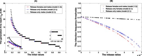
Figure 7. Implications on the design of release strategy. (A) The generation N  to reach $x_N>0.93$ shows a step-like decrease as the increase of the initial values. (B) Under three release strategies, the infection frequency thresholds are monotonically decreasing with respect to the release ratios.