A delay non-autonomous model for the combined effects of fear, prey refuge and additional food for predator

Figures & data

Table 1. Biological meanings of parameters involved in system (1(1) $\begin{array}{rl}\frac{\mathrm{d}N}{\mathrm{d}t}& =\frac{r_{0}N}{1+kP}-r_1{N}^2-\frac{\alpha (1-mP)NP}{\theta +\xi \eta A+b(1-mP)N+cP},\\ \frac{\mathrm{d}P}{\mathrm{d}t}& =\frac{\text{β}\left\{\alpha \right(1-mP)N+\eta A\}P}{\theta +\xi \eta A+b(1-mP)N+cP}-\mathrm{d}P.\end{array}$(1) ) and their values used for numerical simulations.

Parameters	Descriptions	Units	Values
$r_0$	Intrinsic growth rate of prey	1/day	0.7
k	Level of fear responsible for the reduction in the growth rate of prey	unit area/number	0.5
$r_1$	Strength of competition among	unit area/number/day	0.02
	individuals of prey species
α	Consumption rate of predator to prey	1/day	0.74
m	Coefficient of refuge	unit area/number	0.4
A	Amount of additional food	number/unit area	0.2
	to the predators
η	Relative ability of the predator to	1/day	0.4
	detect additional food to prey
ξ	Relative handling time for additional	day	0.3
	food to prey item
b	Proportionality constant	–	0.14
c	Scaling the impact of predator interference	–	0.07
θ	Half saturation value of the predator	number/unit area	0.3
β	Conversion efficiency	–	0.6
d	Death rate of predator	1/day	0.4

Figure 1. Variations of prey (first column) and predator (second column) densities in system (1(1) $\begin{array}{rl}\frac{\mathrm{d}N}{\mathrm{d}t}& =\frac{r_{0}N}{1+kP}-r_1{N}^2-\frac{\alpha (1-mP)NP}{\theta +\xi \eta A+b(1-mP)N+cP},\\ \frac{\mathrm{d}P}{\mathrm{d}t}& =\frac{\text{β}\left\{\alpha \right(1-mP)N+\eta A\}P}{\theta +\xi \eta A+b(1-mP)N+cP}-\mathrm{d}P.\end{array}$(1) ) with respect to (a) k, (b) m and (c) A. Rest of the parameters are at the same values as in Table 1.

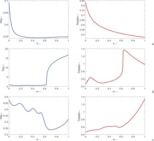
Figure 2. Surface plots of prey (first column) and predator (second column) populations in system (1(1) $\begin{array}{rl}\frac{\mathrm{d}N}{\mathrm{d}t}& =\frac{r_{0}N}{1+kP}-r_1{N}^2-\frac{\alpha (1-mP)NP}{\theta +\xi \eta A+b(1-mP)N+cP},\\ \frac{\mathrm{d}P}{\mathrm{d}t}& =\frac{\text{β}\left\{\alpha \right(1-mP)N+\eta A\}P}{\theta +\xi \eta A+b(1-mP)N+cP}-\mathrm{d}P.\end{array}$(1) ) with respect to (a) m and k, (b) A and k, and (c) A and m. Rest of the parameters are at the same values as in Table 1.

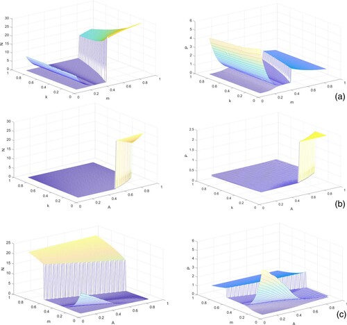
Figure 3. (a) Semi-relative sensitivity and (b) logarithmic sensitivity solutions of system (1(1) $\begin{array}{rl}\frac{\mathrm{d}N}{\mathrm{d}t}& =\frac{r_{0}N}{1+kP}-r_1{N}^2-\frac{\alpha (1-mP)NP}{\theta +\xi \eta A+b(1-mP)N+cP},\\ \frac{\mathrm{d}P}{\mathrm{d}t}& =\frac{\text{β}\left\{\alpha \right(1-mP)N+\eta A\}P}{\theta +\xi \eta A+b(1-mP)N+cP}-\mathrm{d}P.\end{array}$(1) ) with respect to k, m and A. Parameters are at the same values as in Table 1 except m = 0.9 and A = 0.7.

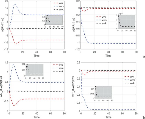
Figure 4. Phase portraits of system (1(1) $\begin{array}{rl}\frac{\mathrm{d}N}{\mathrm{d}t}& =\frac{r_{0}N}{1+kP}-r_1{N}^2-\frac{\alpha (1-mP)NP}{\theta +\xi \eta A+b(1-mP)N+cP},\\ \frac{\mathrm{d}P}{\mathrm{d}t}& =\frac{\text{β}\left\{\alpha \right(1-mP)N+\eta A\}P}{\theta +\xi \eta A+b(1-mP)N+cP}-\mathrm{d}P.\end{array}$(1) ) for $r_0=0.5$, $\alpha =0.36$, $\theta =0.6$ and $\text{β}=0.3$. Rest of the parameters are at the same values as in Table 1 except in (a) $r_1=0.02$, k = m = A = 0, (b) $r_1=0.02$, k = 10, m = A = 0, (c) $r_1=0.02$, m = 0.13, k = A = 0, and (d) $r_1=0.02$, $\xi =0.3$, $\eta =0.4$, A = 7, k = m = 0.

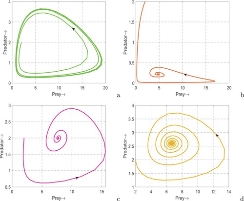
Figure 5. Phase portraits of system (1(1) $\begin{array}{rl}\frac{\mathrm{d}N}{\mathrm{d}t}& =\frac{r_{0}N}{1+kP}-r_1{N}^2-\frac{\alpha (1-mP)NP}{\theta +\xi \eta A+b(1-mP)N+cP},\\ \frac{\mathrm{d}P}{\mathrm{d}t}& =\frac{\text{β}\left\{\alpha \right(1-mP)N+\eta A\}P}{\theta +\xi \eta A+b(1-mP)N+cP}-\mathrm{d}P.\end{array}$(1) ). Parameters are at the same values as in Table 1 except in (a) m = 0.2, (b) k = 0.01, m = 0.2, $\alpha =0.35$, $\xi =0.03$, (c) m = 0.4 and (d) m = 0.2, A = 0.5.

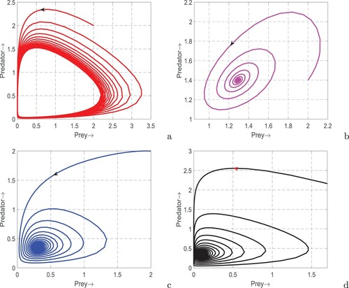
Figure 6. Bifurcation diagram of system (1(1) $\begin{array}{rl}\frac{\mathrm{d}N}{\mathrm{d}t}& =\frac{r_{0}N}{1+kP}-r_1{N}^2-\frac{\alpha (1-mP)NP}{\theta +\xi \eta A+b(1-mP)N+cP},\\ \frac{\mathrm{d}P}{\mathrm{d}t}& =\frac{\text{β}\left\{\alpha \right(1-mP)N+\eta A\}P}{\theta +\xi \eta A+b(1-mP)N+cP}-\mathrm{d}P.\end{array}$(1) ) with respect to (a) k, (b) m and (c) A. Rest of the parameters are at the same values as in Table 1 except in (a) $\xi =0.03$, $\alpha =0.35$, m = 0.2 and (c) m = 0.2.

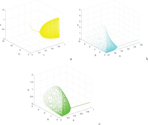
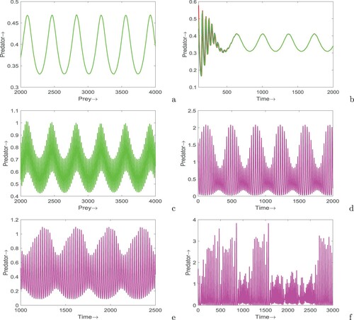
Figure 7. Time series of system (12(12) $\begin{array}{rl}\frac{\mathrm{d}N}{\mathrm{d}t}& =\frac{r_{0}N}{1+kP(t-\tau )}-r_1{N}^2-\frac{\alpha (1-mP)NP}{\theta +\xi \eta A+b(1-mP)N+cP},\\ \frac{\mathrm{d}P}{\mathrm{d}t}& =\frac{\text{β}\left\{\alpha \right(1-mP)N+\eta A\}P}{\theta +\xi \eta A+b(1-mP)N+cP}-\mathrm{d}P.\end{array}$(12) ) for different values of τ: (a) $\tau =4$, (b) $\tau =15$, (c) $\tau =25$ and (d) $\tau =65$. Parameters are at the same values as in Table 1, and the initial conditions are chosen as (2, 1).

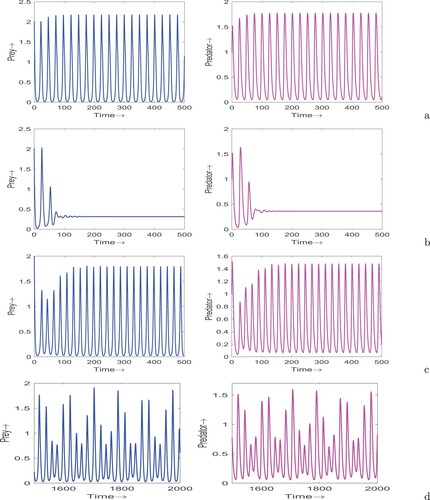
Figure 8. Time series of system (12(12) $\begin{array}{rl}\frac{\mathrm{d}N}{\mathrm{d}t}& =\frac{r_{0}N}{1+kP(t-\tau )}-r_1{N}^2-\frac{\alpha (1-mP)NP}{\theta +\xi \eta A+b(1-mP)N+cP},\\ \frac{\mathrm{d}P}{\mathrm{d}t}& =\frac{\text{β}\left\{\alpha \right(1-mP)N+\eta A\}P}{\theta +\xi \eta A+b(1-mP)N+cP}-\mathrm{d}P.\end{array}$(12) ) for different values of τ: (a) $\tau =4$, (b) $\tau =15$, (c) $\tau =25$ and (d) $\tau =65$. Parameters are at the same values as in Figure 5(a), which shows oscillating behaviour of system (1(1) $\begin{array}{rl}\frac{\mathrm{d}N}{\mathrm{d}t}& =\frac{r_{0}N}{1+kP}-r_1{N}^2-\frac{\alpha (1-mP)NP}{\theta +\xi \eta A+b(1-mP)N+cP},\\ \frac{\mathrm{d}P}{\mathrm{d}t}& =\frac{\text{β}\left\{\alpha \right(1-mP)N+\eta A\}P}{\theta +\xi \eta A+b(1-mP)N+cP}-\mathrm{d}P.\end{array}$(1) ).

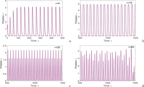
Figure 9. Bifurcation diagram of system (12(12) $\begin{array}{rl}\frac{\mathrm{d}N}{\mathrm{d}t}& =\frac{r_{0}N}{1+kP(t-\tau )}-r_1{N}^2-\frac{\alpha (1-mP)NP}{\theta +\xi \eta A+b(1-mP)N+cP},\\ \frac{\mathrm{d}P}{\mathrm{d}t}& =\frac{\text{β}\left\{\alpha \right(1-mP)N+\eta A\}P}{\theta +\xi \eta A+b(1-mP)N+cP}-\mathrm{d}P.\end{array}$(12) ) with respect to τ. Parameters are at the same values as in Table 1.

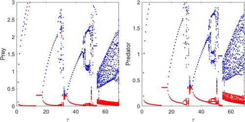
Figure 10. Stability regions for the system (12(12) $\begin{array}{rl}\frac{\mathrm{d}N}{\mathrm{d}t}& =\frac{r_{0}N}{1+kP(t-\tau )}-r_1{N}^2-\frac{\alpha (1-mP)NP}{\theta +\xi \eta A+b(1-mP)N+cP},\\ \frac{\mathrm{d}P}{\mathrm{d}t}& =\frac{\text{β}\left\{\alpha \right(1-mP)N+\eta A\}P}{\theta +\xi \eta A+b(1-mP)N+cP}-\mathrm{d}P.\end{array}$(12) ) in (a) $k-\tau$ and (b) $A-\tau$ planes. Here, blue regions represent the stable coexistence equilibrium for corresponding values of the parameters and green regions represent otherwise. Rest of the parameters are at the same values as in Table 1.

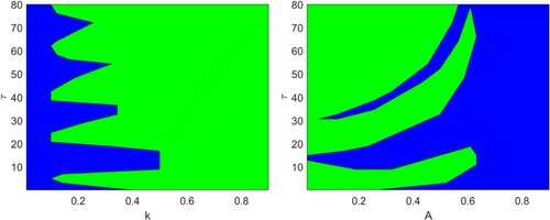
Figure 11. Maximum Lyapunov exponent of the system (12(12) $\begin{array}{rl}\frac{\mathrm{d}N}{\mathrm{d}t}& =\frac{r_{0}N}{1+kP(t-\tau )}-r_1{N}^2-\frac{\alpha (1-mP)NP}{\theta +\xi \eta A+b(1-mP)N+cP},\\ \frac{\mathrm{d}P}{\mathrm{d}t}& =\frac{\text{β}\left\{\alpha \right(1-mP)N+\eta A\}P}{\theta +\xi \eta A+b(1-mP)N+cP}-\mathrm{d}P.\end{array}$(12) ) at $\tau =65$. Parameters are at the same values as in Table 1, and the initial conditions are chosen as (2, 1). In the figure, positive values of the maximum Lyapunov exponent confirm the occurrence of chaotic oscillation.

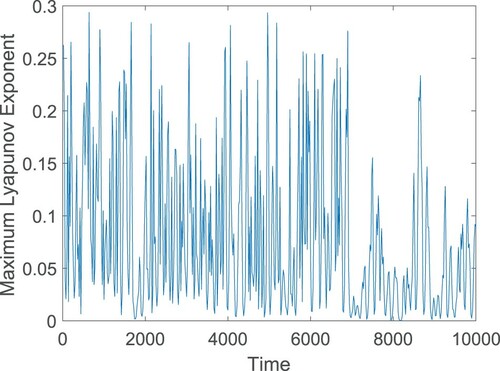
Figure 12. Time series solutions of system (51(51) $\begin{array}{rl}\frac{\mathrm{d}N}{\mathrm{d}t}& =\frac{r_{0}N}{1+k\left(t\right)P(t-\tau )}-r_1{N}^2-\frac{\alpha (1-mP)NP}{\theta +\xi \eta A+b(1-mP)N+cP},\\ \frac{\mathrm{d}P}{\mathrm{d}t}& =\frac{\text{β}\left\{\alpha \right(1-mP)N+\eta A\}P}{\theta +\xi \eta A+b(1-mP)N+cP}-\mathrm{d}P.\end{array}$(51) ) in the absence as well as presence of time delay. Parameters are at the same values as in Table 1, $\omega =2\pi /365$ except in (a) $k_{11}=0.45$, A = 0.6, $\tau =0$, (b) $k_{11}=0.45$, m = 0.2, A = 0.6, $\tau =0$, (c) k = 0.8, $k_{11}=0.4$, $\alpha =0.35$, m = 0.2, $\xi =0.03$, $\tau =0$, (d) $k_{11}=0.4$, $\tau =4$, (e) k = 0.4, $k_{11}=0.35$, $\tau =65$ and (f) $k_{11}=0.4$, m = 0.2, $\tau =65$.