Viability of Pentadesma in reduced habitat ecosystems within two climatic regions with fruit harvesting

Figures & data

Table 1. Description of the variables and parameters of the Pentadesma butyracea model (3(3) $\frac{\mathrm{d}b}{\mathrm{d}t}=\{\begin{array}{ll}{\text{β}}_j(w,\alpha )b\left({\displaystyle 1-\frac{b}{K}}\right)=\left[R_j\right(w,\alpha )-{\mu }_j(w\left)\right]b\left({\displaystyle 1-\frac{b}{K}}\right)& \text{if}\text{β}>0\\ -a{b}^2& \text{if}\text{β}=0\\ {\text{β}}_j(w,\alpha )b\left({\displaystyle 1+\frac{b}{K}}\right)=\left[R_j\right(w,\alpha )-{\mu }_j(w\left)\right]b\left({\displaystyle 1+\frac{b}{K}}\right)& \text{if}\text{β}<0,\end{array}$(3) ).

Variable	Description
$b\left(t\right)$	Density of Pentadesma butyracea tree in a fragment
	of a given width w and a non-lethal harvesting rate α ($\mathrm{\#}$trees/m)
Subscript	Description
j = 1	A dry climatic region
j = 2	A moist climatic region
Parameter	Description
a	The coefficient of the mortality due to competition ($m\times (\text{year}\times \mathrm{\#}\text{trees}{)}^{-1}$).
α	The percentage of Pentadesma's fruits harvested per year (% year${}^{-1}$).
$\text{β}(w,\alpha )$	The net growth rate of the tree population (year${}^{-1}$).
w	The width of the habitat (m).
$R_j(w,\alpha )$	The recruitment rate of new trees into the habitat in the climatic region j (year${}^{-1}$).
${\mu }_j\left(w\right)$	The natural death rate of the population in the climatic region j (year${}^{-1}$).
K	The carrying capacity of the habitat ($\mathrm{\#}$trees/m ).

Figure 1. The function $R_j(w,\alpha )$ defined as in (11(11) $R_j(w,\alpha )=R_o[1-\exp (-(100-\alpha )/{\alpha }_o)][1-\exp (-w/w_o)].$(11) ) with the width expressed in m and $R_j,\alpha$ in year${}^{-1}.$ The surface represents the fitted function. The star marker represents the data points. (a) Dry region (j = 1); and (b) Moist region (j = 2).

Table 2. The values of the parameters and the Fit Standard Error, RMSE, obtained when the fitting of the function $R_j(w,\alpha )$ in Equation (11(11) $R_j(w,\alpha )=R_o[1-\exp (-(100-\alpha )/{\alpha }_o)][1-\exp (-w/w_o)].$(11) ) is performed for moist and dry regions. The values of $R_n$ were computed using formula (12(12) $R_n=R_o[1-\exp (-100/{\alpha }_o)].$(12) ) and the estimated values of the parameters ${\alpha }_o{R}_o,w_o.$

			j = 1 (Dry)		j = 2 (Moist)
Parameter	Description	Unit	Value	RMSE	Value	RMSE
${\alpha }_o$	The harvesting decay constant	year${}^{-1}$	77.52		0.2543
$R_o$	The coefficient of the natural recruitment rate	year${}^{-1}$	0.5544	0.1042	0.2529	0.2253
$w_o$	The width decay constant	m	0.06634		0.8143
$R_n$	The natural recruitment rate of the tree	year${}^{-1}$	0.4018		0.2529

Figure 2. Graphs of $\mu \left(w\right)$ in the dry region (left panel) and the moist region (right panel). The solid black line depicts the curve of the total mortality rate of the tree population fitted using Equation (13(13) ${\mu }_j\left(w\right)=(1-{\mu }_{F_j})\mathrm{e}\mathrm{x}\mathrm{p}(-d_{j}w)+{\mu }_{F_j},j=1,2,$(13) ). The corresponding data values are indicated with a circle symbol. The blue circle shown in the right panel indicates an outlier. The width is expressed in m and μ is in year${}^{-1}.$

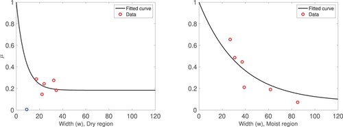
Table 3. Values of the parameter $d_j,$ in metres, when the functions ${\mu }_j$ in Equations (13(13) ${\mu }_j\left(w\right)=(1-{\mu }_{F_j})\mathrm{e}\mathrm{x}\mathrm{p}(-d_{j}w)+{\mu }_{F_j},j=1,2,$(13) ) is fitted to data. The subscripts j = 1, 2 denote dry and moist region, respectively. The subscripts j in the different quantities were dropped to make the table easier to read.

j = 1		j = 2
${\mu }_F$	d (RMSE)	${\mu }_F$	$d_{}$ (RMSE)
0.1832	$0.1320\left(0.05974\right)$	0.07207	$0.0288\left(0.1120\right)$

Figure 3. The graphs of the net growth rate ${\text{β}}_j(w,\alpha ),j=1,2$ of the tree population defined in (2(2) ${\text{β}}_j(w,\alpha )=R_j(w,\alpha )-{\mu }_j\left(w\right),$(2) ). The width is expressed in m, and ${\text{β}}_j,\alpha$ in year${}^{-1}.$ (left) Dry region, $j=1.$ (right) Moist region, $j=2.$

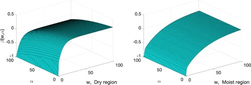
Figure 4. Critical harvesting rate ${\alpha }_c$ as a function of habitat width $w_c.$ The dashed black line corresponds to ${\alpha }_c\left(w_c\right)$ in the dry region while the solid blue line corresponds to ${\alpha }_c\left(w_c\right)$ in the moist region. The quantity α is expressed in % per year and the width in metres.

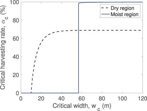
Table 4. Values of the critical harvesting rate ${\alpha }_c$ for each habitat in the two climatic regions of Benin.

Dry region			Moist region
Site	Width (m)	${\alpha }_c$ (% year${}^{-1})$	Site	Width (m)	${\alpha }_c$ (% year${}^{-1})$
Gbasse	9	0	Gouta	26.9	0
Kouba	17.33	49.3	Guiguisso	30.83	0
Tchoundekou	22.2	59.2	Kpiti	37.25	0
Peperkou	24	61.4	Setou	39	0
Kota	32.33	66.5	Alem	61.67	99.4
Tandafa	34.5	67.1	Bakabaka	85.13	99.8

Table 5. Values of the critical habitat width $w_c$ for each current non-lethal harvesting level observed in the two climatic regions of Benin.

Dry region			Moist region
Site	α (% year${}^{-1}$)	$w_c\left(m\right)$	Site	α (% year${}^{-1}$)	$w_c\left(m\right)$
Gbasse	0	10.0	Kpiti	2.5	56.8
Kota	0	10.0	Alem	$25.15$	56.8
Tandafa	43.7	15.7	Bakabaka	33.81	56.8
Tchoundekou	76.5	−	Setou	64.13	56.8
Peperkou	82.2	−	Guiguisso	81.74	56.8
Kouba	89.05	−	Gouta	87.97	56.8

Figure 5. Number of Pentadesma trees per width, b, as a function of time (years) with $b\left(0\right)=\mathrm{0.20.}$ The width w is expressed in m. The distinct values of the width considered in the simulations are shown in the figure and $\alpha =50,65,70\mathrm{\%}$ per year. (a) Dry region of Benin. (b) Moist region of Benin.

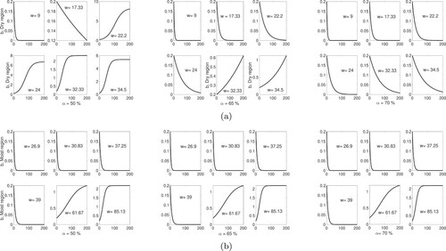
Table 6. Description of functions in Equation (14(14) $\begin{array}{rl}N(t+\mathrm{\Delta }t)& =N\left(t\right)+N_f\left(t\right)-N_h\left(t\right)-N_s\left(t\right),\\ N\left(0\right)& =0,t\in [0,T].\end{array}$(14) ).

Quantities	Description
$N\left(t\right)$	The total number of fruits on the ground at time t
$N_f\left(t\right)$	The number of fruits fallen from a single Pentadesma tree
$N_h\left(t\right)$	The number of harvested fruits from a single tree
$N_s\left(t\right)$	The number of stolen or lost fruits that falls from a single tree
$r_f\left(t\right)$	Rate at which the fruits are dropping
$r\left(t\right)$	Harvesting rate of the fallen fruits
$r_s\left(t\right)$	Rate at which the fruits are stolen or lost

Figure 6. Plots for scenarios varying the cost constant c. Left panel, Number of fruits. Right panel, Harvesting rate. $\gamma =0.1$, $N_{max}=100,$ $c=1,5,10$ and 100. Time t = 0 is the time when the first fruits fall to the ground.

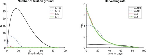
Figure 7. Plots for scenario varying the amount of fruits lost or stolen $\gamma =0,0.05$ and 0.1, and setting $c=10,N_{max}=100$. Left panel, Number of fruits. Right panel, Harvesting rate. Time t = 0 corresponds to the time when the first fruits fall to the ground. The case c = 10 and $\gamma =0.1$ corresponds to a case when we varied the cost constant c considered in Figure 6 and is included for completeness.

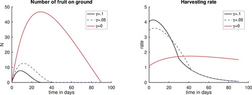
Figure 8. Plots for scenarios varying $N_{\mathrm{m}\mathrm{a}\mathrm{x}}$, and setting $c=10,\gamma =0.1$, and $N_{max}=50,150,200$ and 400. Left panel, Number of fruits. Right panel, Harvesting rate. Time t = 0 is the time when the first fruits fall to the ground. The case c = 10 and $\gamma =0.1$ corresponds to a case when we varied the cost constant c considered in Figure 6 and is included for completeness.

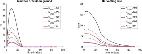
Figure 9. Plots varying the number of fruits left on the ground N_l. Left panel, Number of fruits. Right panel, Harvesting rate. $c=10,\gamma =0,N_{max}=100$ and $N_l=0$; $N_{max}=98$ and $N_l=2$; $N_{max}=95$ and $N_l=5$; $N_{max}=90$ and $N_l=10$. Observe that the first case correspond to one of the cases preseted in Figure 6. Time t = 0 corresponds to the time when the first fruits fall to the ground.

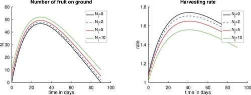
Table A1. For each climatic region of Benin and each habitat the following values are provided: the width of the habitat, the harvesting rate implemented, the number of offspring trees in years 2016 and 2017. For each site a single value is given for the total number of trees in the population.

				Offsprings ( $\mathrm{\#}$ individuals)
Region j	Site (m)	Width w (% year${}^{-1}$)	Harvesting rate α (year${}^{-1}$)	2016	2017	Total population( # trees)
1 (Dry)	Gbasse	9	0	18	0	20
	Kota	32.33	0	20	23	54
	Kouba	17.33	89.05	39	18	145
	Peperkou	24	82.2	16	19	144
	Tandafa	34.5	43.74	38	16	159
	Tchoundekou	22.2	76.5	49	8	156
2 (Moist)	Alem	61.67	25.15	14	4	68
	Bakabaka	85.13	33.81	19	37	158
	Gouta	26.9	87.97	39	11	63
	Guiguisso	30.83	81.74	31	17	137
	Kpiti	37.25	2.5	81	89	158
	Setou	39	64.13	25	27	265

Table A2. The value of the Pentadesma recruitment rate for each habitat within each climatic region.

Region j	Site	Width w (m )	Recruitment rate (% year${}^{-1}$ )
1 (Dry)	Gbasse	9	0.45000
	Kota	32.33	0.39815
	Kouba	17.33	0.19655
	Peperkou	24	0.12153
	Tandafa	34.5	0.16982
	Tchoundekou	22.2	0.18269
2 (Moist)	Alem	61.67	0.13235
	Bakabaka	85.13	0.17722
	Gouta	26.9	0.39683
	Guiguisso	30.83	0.17518
	Kpiti	37.25	0.53797
	Setou	39	0.09811

Table A3. The values of the mortality rate in the dry (j = 1) and moist (j = 2) region of Benin for offsprings and adult trees. The experimental values are given for 2016 and 2017.

			Mortality rate (year${}^{-1}$)
			Offsprings		Adults		Total mortality
Region j	Site	Width	2016	2017	2016	2017	Average
1 (Dry)	Gbasse	9	0.01064	0	0	0	0.0053
	Kota	32.33	0.32331	0.08287	0.10714	0.03774	0.2755
	Kouba	17.33	0.38571	0.11538	0.06623	0.00685	0.2871
	Peperkou	24	0.07921	0.14458	0.15842	0.10390	0.2430
	Tandafa	34.5	0.14238	0.10870	0.06857	0.046781	0.1832
	Tchoundekou	32.33	0.12376	0.16770	0	0	0.1457
2 (Moist)	Alem	61.67	0.13187	0.17822	0.05634	0.01471	0.1905
	Bakabaka	85.13	0.02365	0.10769	0.00685	0.00595	0.07207
	Gouta	26.9	0.34568	0.57031	0.23864	0.15517	0.6549
	Guiguisso	30.83	0.22876	0.34470	0.18182	0.21600	0.4856
	Kpiti	37.25	0.29399	0.545820	0.03311	0.01987	0.4464
	Setou	39	0.16279	0.19937	0.05592	0.00386	0.2110

Table A4. The total natural death rate ${\mu }_{F_j}$ of the Pentadesma tree within each climatic region.

Region j	Maximum width, w	${\mu }_{F_j}$
1	34.5	0.1832
2	85.13	0.07207