Deciphering the transmission dynamics of COVID-19 in India: optimal control and cost effective analysis

Figures & data

Figure 1. Flow diagram of model (1(1) $\begin{array}{rl}\frac{\mathrm{d}{S}_u}{\mathrm{d}t}& =\mathrm{\Lambda }-\lambda S_u-\mathrm{d}{S}_u-q{S}_u+\zeta S_q,\\ \frac{\mathrm{d}{S}_q}{\mathrm{d}t}& =q{S}_u+(1-p)\lambda S_u-({ϵ}_q\lambda +\zeta +d)S_q,\\ \frac{\mathrm{d}E}{\mathrm{d}t}& =p\lambda S_u+{ϵ}_q\lambda S_q-(\alpha +d)E,\\ \frac{\mathrm{d}{I}_a}{\mathrm{d}t}& =p_1\alpha E-({\delta }_1+{\varphi }_1+{\gamma }_1+d)I_a,\\ \frac{\mathrm{d}I}{\mathrm{d}t}& =p_2\alpha E-({\delta }_2+{\varphi }_2+{\gamma }_2+d)I,\\ \frac{\mathrm{d}{I}_h}{\mathrm{d}t}& =(1-p_1-p_2)\alpha E+{\varphi }_1{I}_a+{\varphi }_{2}I-({\delta }_3+{\gamma }_3+d)I_h,\\ \frac{\mathrm{d}R}{\mathrm{d}t}& ={\gamma }_1{I}_a+{\gamma }_{2}I+{\gamma }_3{I}_h-\mathrm{d}R,\end{array}$(1) ).

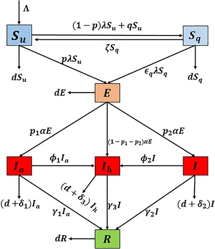
Table 1. Biological interpretation of the model parameters used in system (1(1) $\begin{array}{rl}\frac{\mathrm{d}{S}_u}{\mathrm{d}t}& =\mathrm{\Lambda }-\lambda S_u-\mathrm{d}{S}_u-q{S}_u+\zeta S_q,\\ \frac{\mathrm{d}{S}_q}{\mathrm{d}t}& =q{S}_u+(1-p)\lambda S_u-({ϵ}_q\lambda +\zeta +d)S_q,\\ \frac{\mathrm{d}E}{\mathrm{d}t}& =p\lambda S_u+{ϵ}_q\lambda S_q-(\alpha +d)E,\\ \frac{\mathrm{d}{I}_a}{\mathrm{d}t}& =p_1\alpha E-({\delta }_1+{\varphi }_1+{\gamma }_1+d)I_a,\\ \frac{\mathrm{d}I}{\mathrm{d}t}& =p_2\alpha E-({\delta }_2+{\varphi }_2+{\gamma }_2+d)I,\\ \frac{\mathrm{d}{I}_h}{\mathrm{d}t}& =(1-p_1-p_2)\alpha E+{\varphi }_1{I}_a+{\varphi }_{2}I-({\delta }_3+{\gamma }_3+d)I_h,\\ \frac{\mathrm{d}R}{\mathrm{d}t}& ={\gamma }_1{I}_a+{\gamma }_{2}I+{\gamma }_3{I}_h-\mathrm{d}R,\end{array}$(1) ).

Parameter	Biological interpretation
Λ	Requirement rate
β	Transmission coefficient in the absence of control measures
$p_M$	Proportion of individuals who use face-masks in public
${ϵ}_M$	Measure the effectiveness of face- masks in avoiding COVID-19 infection
p	Proportion of individuals who become exposed after a contact with an infectious individual.
d	The natural death rate of individuals
ζ	Rate at which the quarantined individuals go back to susceptible class $(S_u)$
${ϵ}_q$	Measures the efficacy of quarantine to avert COVID-19 transmission during quarantine
${\psi }_a({\psi }_h)$	Modification factor for the infectiousness of asymptomatically (isolated) infectious individuals
${ϵ}_h$	Measures the effectiveness of isolation in preventing the transmission of COVID-19 disease in a hospital or isolation site.
$\frac{1}{\alpha }$	Incubation period for exposed individuals
$p_1(p_2)$	Proportion of exposed individuals who enter to the $I_a(I)$ classes after the incubation period
$1-(p_1+p_2)$	Proportion of exposed individuals who move to the $I_h$ class at the end the incubation period (after diagnosed)
${\delta }_1({\delta }_2)({\delta }_3)$	COVID-19 infection induced death rate of individuals in the $I_a(I)(I_h)$ classes
${\gamma }_1({\gamma }_2)({\gamma }_3)$	Recovery rate for the $I_a(I)(I_h)$ classes
${\varphi }_1({\varphi }_2)$	Isolation/hospitalization rate for individuals in the $I_a(I)$ classes after diagnosis

Figure 2. The figure shows the bifurcation analysis discussed in Section 3.4.1. (a) backward bifurcation when imperfect quarantine is implemented $({ϵ}_q\ne 0)$ and (b) backward bifurcation when perfect quarantine is implemented $({ϵ}_q=0)$.

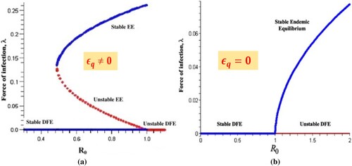
Figure 3. (a) The histogram of MCMC chain for parameters β and $p_M$ with 100, 000 sample realizations. (b) Fitting results of reported cases for India to the model output.

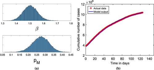
Table 2. The estimated values of model parameters $\beta \mathrm{and}{p}_M$ with its $95\mathrm{\%}$ confidence interval obtained via MCMC method.

Parameters	Mean values	Standard deviations	$95\mathrm{\%}$ CI	Geweke values
β	1.5030	0.0524	$(1.3982,1.6078)$	0.9972
$p_M$	0.2728	0.0486	$(0.1756,0.3700)$	0.9958

Table 3. Initial conditions for the system (1(1) $\begin{array}{rl}\frac{\mathrm{d}{S}_u}{\mathrm{d}t}& =\mathrm{\Lambda }-\lambda S_u-\mathrm{d}{S}_u-q{S}_u+\zeta S_q,\\ \frac{\mathrm{d}{S}_q}{\mathrm{d}t}& =q{S}_u+(1-p)\lambda S_u-({ϵ}_q\lambda +\zeta +d)S_q,\\ \frac{\mathrm{d}E}{\mathrm{d}t}& =p\lambda S_u+{ϵ}_q\lambda S_q-(\alpha +d)E,\\ \frac{\mathrm{d}{I}_a}{\mathrm{d}t}& =p_1\alpha E-({\delta }_1+{\varphi }_1+{\gamma }_1+d)I_a,\\ \frac{\mathrm{d}I}{\mathrm{d}t}& =p_2\alpha E-({\delta }_2+{\varphi }_2+{\gamma }_2+d)I,\\ \frac{\mathrm{d}{I}_h}{\mathrm{d}t}& =(1-p_1-p_2)\alpha E+{\varphi }_1{I}_a+{\varphi }_{2}I-({\delta }_3+{\gamma }_3+d)I_h,\\ \frac{\mathrm{d}R}{\mathrm{d}t}& ={\gamma }_1{I}_a+{\gamma }_{2}I+{\gamma }_3{I}_h-\mathrm{d}R,\end{array}$(1) ).

$S_u(0)$	$S_q(0)$	$E(0)$	$I_a(0)$	$I(0)$	$I_h(0)$	$R(0)$
$1.35\times {10}^9$	$1.15\times {10}^7$	$2.76\times {10}^6$	$6.6\times {10}^5$	$9.42\times {10}^4$	$1.89\times {10}^5$	$2.96\times {10}^6$

Table 4. The table contains numerical values of model parameters used for transmission dynamics of system (1(1) $\begin{array}{rl}\frac{\mathrm{d}{S}_u}{\mathrm{d}t}& =\mathrm{\Lambda }-\lambda S_u-\mathrm{d}{S}_u-q{S}_u+\zeta S_q,\\ \frac{\mathrm{d}{S}_q}{\mathrm{d}t}& =q{S}_u+(1-p)\lambda S_u-({ϵ}_q\lambda +\zeta +d)S_q,\\ \frac{\mathrm{d}E}{\mathrm{d}t}& =p\lambda S_u+{ϵ}_q\lambda S_q-(\alpha +d)E,\\ \frac{\mathrm{d}{I}_a}{\mathrm{d}t}& =p_1\alpha E-({\delta }_1+{\varphi }_1+{\gamma }_1+d)I_a,\\ \frac{\mathrm{d}I}{\mathrm{d}t}& =p_2\alpha E-({\delta }_2+{\varphi }_2+{\gamma }_2+d)I,\\ \frac{\mathrm{d}{I}_h}{\mathrm{d}t}& =(1-p_1-p_2)\alpha E+{\varphi }_1{I}_a+{\varphi }_{2}I-({\delta }_3+{\gamma }_3+d)I_h,\\ \frac{\mathrm{d}R}{\mathrm{d}t}& ={\gamma }_1{I}_a+{\gamma }_{2}I+{\gamma }_3{I}_h-\mathrm{d}R,\end{array}$(1) ) for COVID-19 in India.

Parameters	Numerical value	Units	References
Γ	0	day${}^{-1}$	Assumed
${ϵ}_M$	0.6		[28, 29, 63, 68]
${\psi }_a$	0.49		[46]
${\psi }_h$	0.35		assumed
${ϵ}_h$	0.2		assumed
d	0	day${}^{-1}$	assumed
q	0.25		assumed
ζ	$\frac{1}{14}$	day${}^{-1}$	[71, 73]
p	0.36651		assumed
${ϵ}_q$	0.2		assumed
α	0.1980	day${}^{-1}$	[45]
$p_1$	0.4		[4, 31]
$p_2$	0.2		[4, 31]
${\delta }_1$	0.0019	day${}^{-1}$	assumed
${\delta }_2$	0.0019	day${}^{-1}$	assumed
${\delta }_3$	0.0018	day${}^{-1}$	assumed
${\gamma }_1$	0.1	day${}^{-1}$	[32, 82]
${\gamma }_2$	0.1	day${}^{-1}$	[32, 82]
${\gamma }_3$	0.125	day${}^{-1}$	[32, 82]
${\varphi }_1$	0.456	day${}^{-1}$	assumed
${\varphi }_2$	0.2	day${}^{-1}$	[32]

Figure 4. The long-term dynamics of the model system (1(1) $\begin{array}{rl}\frac{\mathrm{d}{S}_u}{\mathrm{d}t}& =\mathrm{\Lambda }-\lambda S_u-\mathrm{d}{S}_u-q{S}_u+\zeta S_q,\\ \frac{\mathrm{d}{S}_q}{\mathrm{d}t}& =q{S}_u+(1-p)\lambda S_u-({ϵ}_q\lambda +\zeta +d)S_q,\\ \frac{\mathrm{d}E}{\mathrm{d}t}& =p\lambda S_u+{ϵ}_q\lambda S_q-(\alpha +d)E,\\ \frac{\mathrm{d}{I}_a}{\mathrm{d}t}& =p_1\alpha E-({\delta }_1+{\varphi }_1+{\gamma }_1+d)I_a,\\ \frac{\mathrm{d}I}{\mathrm{d}t}& =p_2\alpha E-({\delta }_2+{\varphi }_2+{\gamma }_2+d)I,\\ \frac{\mathrm{d}{I}_h}{\mathrm{d}t}& =(1-p_1-p_2)\alpha E+{\varphi }_1{I}_a+{\varphi }_{2}I-({\delta }_3+{\gamma }_3+d)I_h,\\ \frac{\mathrm{d}R}{\mathrm{d}t}& ={\gamma }_1{I}_a+{\gamma }_{2}I+{\gamma }_3{I}_h-\mathrm{d}R,\end{array}$(1) ) when $R_0=0.4951<1.$ The figure ensure the local stability of the disease free equilibrium.

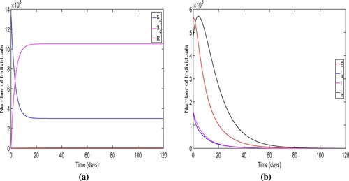
Figure 5. The long-term dynamics of the model system (1(1) $\begin{array}{rl}\frac{\mathrm{d}{S}_u}{\mathrm{d}t}& =\mathrm{\Lambda }-\lambda S_u-\mathrm{d}{S}_u-q{S}_u+\zeta S_q,\\ \frac{\mathrm{d}{S}_q}{\mathrm{d}t}& =q{S}_u+(1-p)\lambda S_u-({ϵ}_q\lambda +\zeta +d)S_q,\\ \frac{\mathrm{d}E}{\mathrm{d}t}& =p\lambda S_u+{ϵ}_q\lambda S_q-(\alpha +d)E,\\ \frac{\mathrm{d}{I}_a}{\mathrm{d}t}& =p_1\alpha E-({\delta }_1+{\varphi }_1+{\gamma }_1+d)I_a,\\ \frac{\mathrm{d}I}{\mathrm{d}t}& =p_2\alpha E-({\delta }_2+{\varphi }_2+{\gamma }_2+d)I,\\ \frac{\mathrm{d}{I}_h}{\mathrm{d}t}& =(1-p_1-p_2)\alpha E+{\varphi }_1{I}_a+{\varphi }_{2}I-({\delta }_3+{\gamma }_3+d)I_h,\\ \frac{\mathrm{d}R}{\mathrm{d}t}& ={\gamma }_1{I}_a+{\gamma }_{2}I+{\gamma }_3{I}_h-\mathrm{d}R,\end{array}$(1) ) when $R_0=0.9529<1.$ The figure ensure the local stability of a EE when $R_0<1$.

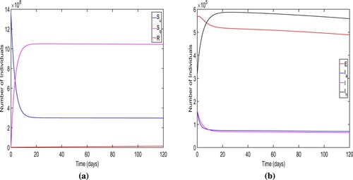
Figure 6. The long-term dynamics of the solutions of model system (1(1) $\begin{array}{rl}\frac{\mathrm{d}{S}_u}{\mathrm{d}t}& =\mathrm{\Lambda }-\lambda S_u-\mathrm{d}{S}_u-q{S}_u+\zeta S_q,\\ \frac{\mathrm{d}{S}_q}{\mathrm{d}t}& =q{S}_u+(1-p)\lambda S_u-({ϵ}_q\lambda +\zeta +d)S_q,\\ \frac{\mathrm{d}E}{\mathrm{d}t}& =p\lambda S_u+{ϵ}_q\lambda S_q-(\alpha +d)E,\\ \frac{\mathrm{d}{I}_a}{\mathrm{d}t}& =p_1\alpha E-({\delta }_1+{\varphi }_1+{\gamma }_1+d)I_a,\\ \frac{\mathrm{d}I}{\mathrm{d}t}& =p_2\alpha E-({\delta }_2+{\varphi }_2+{\gamma }_2+d)I,\\ \frac{\mathrm{d}{I}_h}{\mathrm{d}t}& =(1-p_1-p_2)\alpha E+{\varphi }_1{I}_a+{\varphi }_{2}I-({\delta }_3+{\gamma }_3+d)I_h,\\ \frac{\mathrm{d}R}{\mathrm{d}t}& ={\gamma }_1{I}_a+{\gamma }_{2}I+{\gamma }_3{I}_h-\mathrm{d}R,\end{array}$(1) ) when $R_0=1.3649>1.$ The figure ensure the local stability of a endemic equilibrium when $R_0>1$.

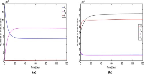
Figure 7. The figure represents the normalized forward sensitivity index for the $R_0$ given in Equation (4(4) $R_0=R_0^I+R_0^{I_a}+R_0^{I_h},$(4) ).

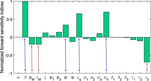
Figure 8. The figure depicts the PRCCs for the basic reproduction number $R_0$ given in Equation (4(4) $R_0=R_0^I+R_0^{I_a}+R_0^{I_h},$(4) ).

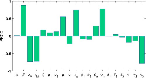
Figure 9. The figure depicts the threshold dynamics of $R_0$ discussed in Section 3.5.

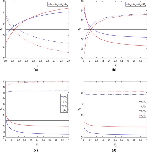
Figure 10. The figure depicts the impact of important model parameters on the $R_0$ for model system (1(1) $\begin{array}{rl}\frac{\mathrm{d}{S}_u}{\mathrm{d}t}& =\mathrm{\Lambda }-\lambda S_u-\mathrm{d}{S}_u-q{S}_u+\zeta S_q,\\ \frac{\mathrm{d}{S}_q}{\mathrm{d}t}& =q{S}_u+(1-p)\lambda S_u-({ϵ}_q\lambda +\zeta +d)S_q,\\ \frac{\mathrm{d}E}{\mathrm{d}t}& =p\lambda S_u+{ϵ}_q\lambda S_q-(\alpha +d)E,\\ \frac{\mathrm{d}{I}_a}{\mathrm{d}t}& =p_1\alpha E-({\delta }_1+{\varphi }_1+{\gamma }_1+d)I_a,\\ \frac{\mathrm{d}I}{\mathrm{d}t}& =p_2\alpha E-({\delta }_2+{\varphi }_2+{\gamma }_2+d)I,\\ \frac{\mathrm{d}{I}_h}{\mathrm{d}t}& =(1-p_1-p_2)\alpha E+{\varphi }_1{I}_a+{\varphi }_{2}I-({\delta }_3+{\gamma }_3+d)I_h,\\ \frac{\mathrm{d}R}{\mathrm{d}t}& ={\gamma }_1{I}_a+{\gamma }_{2}I+{\gamma }_3{I}_h-\mathrm{d}R,\end{array}$(1) ). The numerical values of all parameter other than (a) $p_M$ and ${ϵ}_M$; (b) ζ and q; (c) ${\psi }_h$ and ${\psi }_a$; (d) ${\varphi }_1$ and ${\varphi }_2$ are given in Tables 2 and 4. (a) Effect of $p_M$ and ${ϵ}_M$ on basic reproduction number $(R_0).$ (b) Effect of ζ and q on basic reproduction number $(R_0).$ (c) Effect of ${\psi }_h$ and ${\psi }_a$ on basic reproduction number $(R_0).$ and (d) Effect of ${\varphi }_1$ and ${\varphi }_2$ on basic reproduction number $(R_0).$

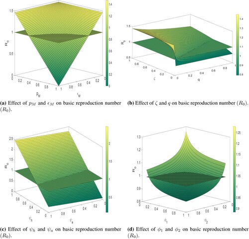
Figure 11. The trajectory of total infectious cases and control profile for the strategy A.

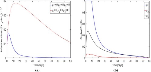
Figure 12. The figure depicts the trajectories of total infectious cases and control profile for the strategy B.

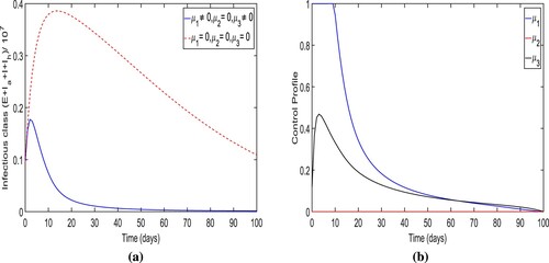
Figure 13. The figure depicts the trajectory of total infectious cases and control profile for the case of strategy C.

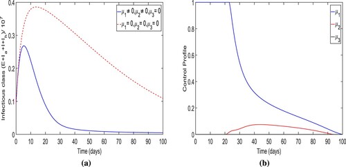
Figure 14. The figure depicts the trajectory of total infectious cases and control profile for the strategy D.

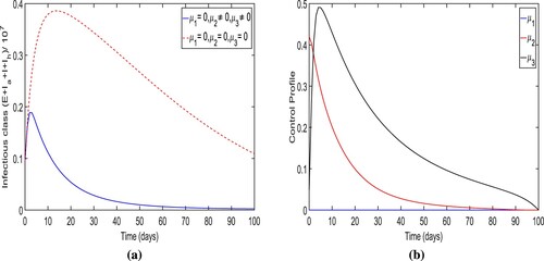
Figure 15. The figure illustrates the optimal trajectory of total infectious cases and control profile for control strategy E.

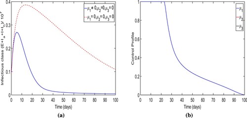
Figure 16. The figure determines the optimal trajectory of total infectious cases and control profile for intervention strategy G.

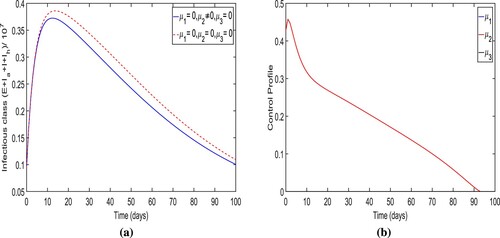
Figure 17. The figure illustrates the trajectories of total infectious cases and control profile for control strategy G.

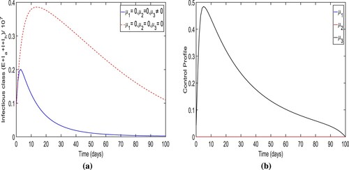
Figure 18. The figure depicts the IAR for all seven optimal control strategies.

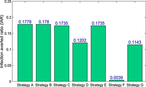
Table 5. Control measures with increasing order of total infection cases avoided.

Strategy	Total infection averted	Total cost	IAR	ACER
$F:{\mu }_2\ne 0$	$2.88\times {10}^7$	35.0031	0.0039	$1.21\times {10}^{-6}$
$G:{\mu }_3\ne 0$	$32.60\times {10}^7$	35.4920	0.1143	$1.08\times {10}^{-7}$
$D:{\mu }_2,{\mu }_3\ne 0$	$33.33\times {10}^7$	40.4781	0.1202	$1.21\times {10}^{-7}$
$C:{\mu }_1,{\mu }_2\ne 0$	$33.73\times {10}^7$	23.9467	0.1735	$7.10\times {10}^{-8}$
$E:{\mu }_1\ne 0$	$33.74\times {10}^7$	20.6084	0.1735	$6.11\times {10}^{-8}$
$B:{\mu }_1,{\mu }_3\ne 0$	$36.66\times {10}^7$	35.3076	0.1780	$9.63\times {10}^{-7}$
$A:{\mu }_1,{\mu }_2,{\mu }_3\ne 0$	$36.70\times {10}^7$	36.7240	0.1779	$1\times {10}^{-7}$

Figure 19. The figure shows the ACER for all seven optimal control strategies.

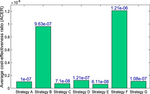
Figure 20. Comparison of all intervention strategies in terms of total cost and number of averted cases.

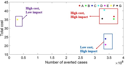
Table 6. ICER computations for strategies F and G.

Strategy	Total infection averted	Total cost	ACER	ICER
F	$2.88\times {10}^7$	35.0031	$1.21\times {10}^{-6}$	$1.21\times {10}^{-6}$
G	$32.60\times {10}^7$	35.4920	$1.08\times {10}^{-7}$	$1.64\times {10}^{-9}$

Table 7. ICER computations for strategies D and G.

Strategy	Total infection averted	Total cost	ACER	ICER
G	$32.60\times {10}^7$	35.4920	$1.08\times {10}^{-7}$	$1.08\times {10}^{-7}$
D	$33.33\times {10}^7$	40.4781	$1.21\times {10}^{-7}$	$6.83\times {10}^{-7}$

Table 8. ICER computations for strategies C and G.

Strategy	Total infection averted	Total cost	ACER	ICER
G	$32.60\times {10}^7$	35.4920	$1.08\times {10}^{-7}$	$1.08\times {10}^{-7}$
C	$33.73\times {10}^7$	23.9467	$7.10\times {10}^{-8}$	$-1.58\times {10}^{-6}$

Table 9. ICER computations for strategies E and C.

Strategy	Total infection averted	Total cost	ACER	ICER
C	$33.73\times {10}^7$	23.9467	$7.10\times {10}^{-8}$	$7.10\times {10}^{-8}$
E	$33.74\times {10}^7$	20.6084	$6.11\times {10}^{-8}$	$-3.33\times {10}^{-8}$

Table 10. ICER computations for strategies E and B.

Strategy	Total infection averted	Total cost	ACER	ICER
E	$33.74\times {10}^7$	20.6084	$6.11\times {10}^{-8}$	$6.11\times {10}^{-8}$
B	$36.66\times {10}^7$	35.3076	$9.63\times {10}^{-7}$	$5.03\times {10}^{-7}$

Table 11. ICER computations for strategies E and A.

Strategy	Total infection averted	Total cost	ACER	ICER
E	$33.74\times {10}^7$	20.6084	$6.11\times {10}^{-8}$	$6.11\times {10}^{-8}$
A	$36.70\times {10}^7$	36.7240	$1\times {10}^{-7}$	$5.44\times {10}^{-7}$

K.V. Driessche, N. Hens, P. Tilley, B.S. Quon, M.A. Chilvers, R. de Groot, M.F. Cotton, B.J. Marais, D.P. Speert, and J.E.A. Zlosnik, Surgical masks reduce airborne spread of Pseudomonas aeruginosa in colonized patients with cystic fibrosis, Am. J. Respir. Crit. Care. Med. 192(7) (2015), pp. 897–899.

 PubMed Web of Science ®Google Scholar

S.E. Eikenberry, M. Mancuso, E. Iboi, T. Phan, K. Eikenberry, Y. Kuang, E. Kostelich, and A.B. Gumel, To mask or not to mask: Modeling the potential for face mask use by the general public to curtail the COVID-19 pandemic, Infect. Dis. Model. 5 (2020), pp. 293–308.

 PubMedGoogle Scholar

R.E. Stockwell, M.E. Wood, C. He, L.J. Sherrard, E.L. Ballard, T.J. Kidd, G.R. Johnson, L.D. Knibbs, and S.C. Bell, Face masks reduce the release of Pseudomonas aeruginosa cough aerosols when worn for clinically relevant periods, Am. J. Respir. Crit. Care. Med. 198(10) (2018), pp. 1339–1342.

 PubMed Web of Science ®Google Scholar

M. Van der Sande, P. Teunis, and R. Sabel, Professional and home-made face masks reduce exposure to respiratory infections among the general population, PLoS. One. 3(7) (2008), pp. e2618.

 PubMed Web of Science ®Google Scholar

R. Li, S. Pei, B. Chen, Y. Song, T. Zhang, W. Yang, and J. Shaman, Substantial undocumented infection facilitates the rapid dissemination of novel coronavirus (SARS-CoV-2), Science 368(6490) (2020), pp. 489–493.

 PubMed Web of Science ®Google Scholar

World Health Organization, Coronavirus disease 2019 (COVID-19): Situation report, 46, WHO, 2020.

 Google Scholar

World Health Organization, Coronavirus disease (COVID-2019) situation reports, WHO, 2020, Available at https://www.who.int/emergencies/diseases/novel-coronavirus-2019/situation-reports. (Accessed 19 March 2020).

 Google Scholar

Q. Li, X. Guan, P. Wu, X. Wang, L. Zhou, Y. Tong, R. Ren, K.S. Leung, E.H. Lau, J.Y. Wong, and X. Xing, Early transmission dynamics in Wuhan, China, of novel coronavirus-infected pneumonia, N. Engl. J. Med. 382 (2020), pp. 1199–1207.

 PubMed Web of Science ®Google Scholar

R.M. Anderson, H. Heesterbeek, D. Klinkenberg, and T.D. Hollingsworth, How will country-based mitigation measures influence the course of the COVID-19 epidemic?, The Lancet 395(10228) (2020), pp. 931–934.

 PubMed Web of Science ®Google Scholar

European Centre for Disease Prevention and Control, Control, Situation update worldwide, ECDC (2020) Available at https://www.ecdc.europa.eu/en/geographical-distribution-2019-ncov-cases. (Accessed 18 March 2020).

 Google Scholar

N. Ferguson, D. Laydon, G. Nedjati-Gilani, N. Imai, K. Ainslie, M. Baguelin, S. Bhatia, A. Boonyasiri, Z.U.L.M.A. Cucunuba Perez, G. Cuomo-Dannenburg, and A. Dighe, Report 9: Impact of non-pharmaceutical interventions (NPIs) to reduce COVID19 mortality and healthcare demand, Imperial College Lond. 10(77482) (2020), pp. 491–497.

 Google Scholar

L. Zou, F. Ruan, M. Huang, L. Liang, H. Huang, Z. Hong, J. Yu, M. Kang, Y. Song, J. Xia, and Q. Guo, SARS-CoV-2 viral load in upper respiratory specimens of infected patients, N. Eng. J. Med. 382(12) (2020), pp. 1177–1179.

 PubMed Web of Science ®Google Scholar