Stationary distribution and global stability of stochastic predator-prey model with disease in prey population

Figures & data

Table 1. Parameters and meaning – predator-prey model with disease in the first prey.

Parameters	Meaning
α	disease transmission coefficient
β	predation rate of infected first prey
m	half saturation constant for infected first prey
γ	intrinsic growth rate of second prey
δ	predation rate of second prey
c	death rate including natural death rate and disease related death rate of the infected first prey
d, e	natural death rate of second prey and predator

Figure 1. (a) This graph shows that the solution curve of deterministic (2(2) $\{\begin{array}{l}{\displaystyle \frac{\mathrm{d}{X}_S}{\mathrm{d}t}}={\displaystyle \frac{\mathrm{\Pi }{X}_S}{a+X_S}}-\alpha X_S{X}_I-b{X}_S,\\ {\displaystyle \frac{\mathrm{d}{X}_I}{\mathrm{d}t}}=\alpha X_S{X}_I-{\displaystyle \frac{\text{β}{X}_{I}Z}{m+\mu X_I+\eta Z}}-c{X}_I,\\ {\displaystyle \frac{\mathrm{d}Y}{\mathrm{d}t}}=\gamma Y-\delta YZ-dY,\\ {\displaystyle \frac{\mathrm{d}Z}{\mathrm{d}t}}=\delta YZ+{\displaystyle \frac{\text{β}{X}_{I}Z}{m+\mu X_I+\eta Z}}-eZ,\end{array}$(2) ) and stochastic system (4(4) $\{\begin{array}{l}{\displaystyle \frac{\mathrm{d}{X}_S}{\mathrm{d}t}}={\displaystyle \frac{\mathrm{\Pi }{X}_S}{a+X_S}}-\alpha X_S{X}_I-b{X}_S+{\sigma }_1{X}_S{B}_1\left(t\right),\\ {\displaystyle \frac{\mathrm{d}{X}_I}{\mathrm{d}t}}=\alpha X_S{X}_I-{\displaystyle \frac{\text{β}{X}_{I}Z}{m+\mu X_I+\eta Z}}-c{X}_I+{\sigma }_2{X}_I{B}_2\left(t\right),\\ {\displaystyle \frac{\mathrm{d}Y}{\mathrm{d}t}}=\gamma Y-\delta YZ-dY+{\sigma }_{3}Y{B}_3\left(t\right),\\ {\displaystyle \frac{\mathrm{d}Z}{\mathrm{d}t}}=\delta YZ+{\displaystyle \frac{\text{β}{X}_{I}Z}{m+\mu X_I+\eta Z}}-eZ+{\sigma }_{4}Z{B}_4\left(t\right).\end{array}$(4) ) with large noise ${\sigma }_1={\sigma }_2=0.06,{\sigma }_3={\sigma }_4=0.03$ and (b) small noise ${\sigma }_1={\sigma }_2=0.03,{\sigma }_3={\sigma }_4=0.01$.

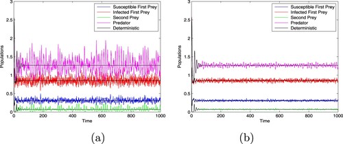
Figure 2. (a) This graph shows that the species of system (2(2) $\{\begin{array}{l}{\displaystyle \frac{\mathrm{d}{X}_S}{\mathrm{d}t}}={\displaystyle \frac{\mathrm{\Pi }{X}_S}{a+X_S}}-\alpha X_S{X}_I-b{X}_S,\\ {\displaystyle \frac{\mathrm{d}{X}_I}{\mathrm{d}t}}=\alpha X_S{X}_I-{\displaystyle \frac{\text{β}{X}_{I}Z}{m+\mu X_I+\eta Z}}-c{X}_I,\\ {\displaystyle \frac{\mathrm{d}Y}{\mathrm{d}t}}=\gamma Y-\delta YZ-dY,\\ {\displaystyle \frac{\mathrm{d}Z}{\mathrm{d}t}}=\delta YZ+{\displaystyle \frac{\text{β}{X}_{I}Z}{m+\mu X_I+\eta Z}}-eZ,\end{array}$(2) ) and (4(4) $\{\begin{array}{l}{\displaystyle \frac{\mathrm{d}{X}_S}{\mathrm{d}t}}={\displaystyle \frac{\mathrm{\Pi }{X}_S}{a+X_S}}-\alpha X_S{X}_I-b{X}_S+{\sigma }_1{X}_S{B}_1\left(t\right),\\ {\displaystyle \frac{\mathrm{d}{X}_I}{\mathrm{d}t}}=\alpha X_S{X}_I-{\displaystyle \frac{\text{β}{X}_{I}Z}{m+\mu X_I+\eta Z}}-c{X}_I+{\sigma }_2{X}_I{B}_2\left(t\right),\\ {\displaystyle \frac{\mathrm{d}Y}{\mathrm{d}t}}=\gamma Y-\delta YZ-dY+{\sigma }_{3}Y{B}_3\left(t\right),\\ {\displaystyle \frac{\mathrm{d}Z}{\mathrm{d}t}}=\delta YZ+{\displaystyle \frac{\text{β}{X}_{I}Z}{m+\mu X_I+\eta Z}}-eZ+{\sigma }_{4}Z{B}_4\left(t\right).\end{array}$(4) ) goes to extinction and (b) each species in both system goes to permanent.

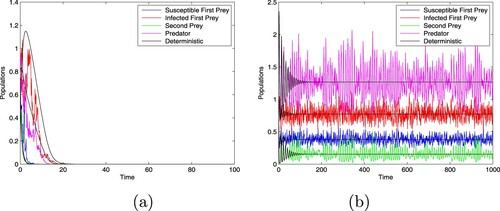
Figure 3. This graph shows the stochastic stability of the system (4(4) $\{\begin{array}{l}{\displaystyle \frac{\mathrm{d}{X}_S}{\mathrm{d}t}}={\displaystyle \frac{\mathrm{\Pi }{X}_S}{a+X_S}}-\alpha X_S{X}_I-b{X}_S+{\sigma }_1{X}_S{B}_1\left(t\right),\\ {\displaystyle \frac{\mathrm{d}{X}_I}{\mathrm{d}t}}=\alpha X_S{X}_I-{\displaystyle \frac{\text{β}{X}_{I}Z}{m+\mu X_I+\eta Z}}-c{X}_I+{\sigma }_2{X}_I{B}_2\left(t\right),\\ {\displaystyle \frac{\mathrm{d}Y}{\mathrm{d}t}}=\gamma Y-\delta YZ-dY+{\sigma }_{3}Y{B}_3\left(t\right),\\ {\displaystyle \frac{\mathrm{d}Z}{\mathrm{d}t}}=\delta YZ+{\displaystyle \frac{\text{β}{X}_{I}Z}{m+\mu X_I+\eta Z}}-eZ+{\sigma }_{4}Z{B}_4\left(t\right).\end{array}$(4) ) around the positive equilibrium with different initial values and ${\sigma }_1=0.04,{\sigma }_2=0.03,{\sigma }_3=0.02,{\sigma }_4=0.01$.

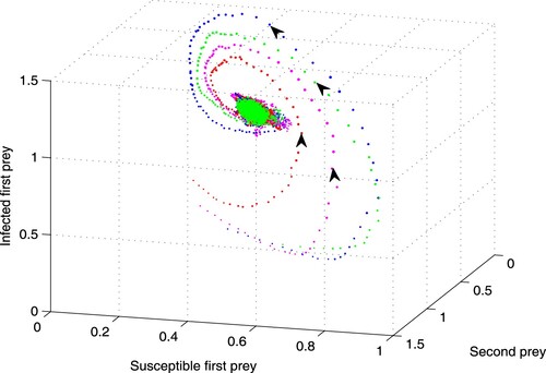
Figure 4. The phase trajectories clearly shows the stochastic stability of individual species in the system (4(4) $\{\begin{array}{l}{\displaystyle \frac{\mathrm{d}{X}_S}{\mathrm{d}t}}={\displaystyle \frac{\mathrm{\Pi }{X}_S}{a+X_S}}-\alpha X_S{X}_I-b{X}_S+{\sigma }_1{X}_S{B}_1\left(t\right),\\ {\displaystyle \frac{\mathrm{d}{X}_I}{\mathrm{d}t}}=\alpha X_S{X}_I-{\displaystyle \frac{\text{β}{X}_{I}Z}{m+\mu X_I+\eta Z}}-c{X}_I+{\sigma }_2{X}_I{B}_2\left(t\right),\\ {\displaystyle \frac{\mathrm{d}Y}{\mathrm{d}t}}=\gamma Y-\delta YZ-dY+{\sigma }_{3}Y{B}_3\left(t\right),\\ {\displaystyle \frac{\mathrm{d}Z}{\mathrm{d}t}}=\delta YZ+{\displaystyle \frac{\text{β}{X}_{I}Z}{m+\mu X_I+\eta Z}}-eZ+{\sigma }_{4}Z{B}_4\left(t\right).\end{array}$(4) ) with different initial values and with the noise ${\sigma }_1=0.04,{\sigma }_2=0.03,{\sigma }_3=0.02,{\sigma }_4=0.01$ converges to the region where the positive equilibrium occur.

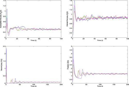
Figure 5. The left panel shows the solution trajectories of both deterministic and stochastic systems from one simulation run; the right panel shows the stationary distribution of each species in the system (4(4) $\{\begin{array}{l}{\displaystyle \frac{\mathrm{d}{X}_S}{\mathrm{d}t}}={\displaystyle \frac{\mathrm{\Pi }{X}_S}{a+X_S}}-\alpha X_S{X}_I-b{X}_S+{\sigma }_1{X}_S{B}_1\left(t\right),\\ {\displaystyle \frac{\mathrm{d}{X}_I}{\mathrm{d}t}}=\alpha X_S{X}_I-{\displaystyle \frac{\text{β}{X}_{I}Z}{m+\mu X_I+\eta Z}}-c{X}_I+{\sigma }_2{X}_I{B}_2\left(t\right),\\ {\displaystyle \frac{\mathrm{d}Y}{\mathrm{d}t}}=\gamma Y-\delta YZ-dY+{\sigma }_{3}Y{B}_3\left(t\right),\\ {\displaystyle \frac{\mathrm{d}Z}{\mathrm{d}t}}=\delta YZ+{\displaystyle \frac{\text{β}{X}_{I}Z}{m+\mu X_I+\eta Z}}-eZ+{\sigma }_{4}Z{B}_4\left(t\right).\end{array}$(4) ) separately from 10,000 simulation runs with intensity of noise ${\sigma }_1={\sigma }_2=0.03,{\sigma }_3={\sigma }_4=0.01$.

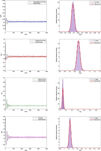
Figure 6. The left panel represents the solution trajectories of both system from one simulation run; the right panel represents the stationary distribution of each species in the system (4(4) $\{\begin{array}{l}{\displaystyle \frac{\mathrm{d}{X}_S}{\mathrm{d}t}}={\displaystyle \frac{\mathrm{\Pi }{X}_S}{a+X_S}}-\alpha X_S{X}_I-b{X}_S+{\sigma }_1{X}_S{B}_1\left(t\right),\\ {\displaystyle \frac{\mathrm{d}{X}_I}{\mathrm{d}t}}=\alpha X_S{X}_I-{\displaystyle \frac{\text{β}{X}_{I}Z}{m+\mu X_I+\eta Z}}-c{X}_I+{\sigma }_2{X}_I{B}_2\left(t\right),\\ {\displaystyle \frac{\mathrm{d}Y}{\mathrm{d}t}}=\gamma Y-\delta YZ-dY+{\sigma }_{3}Y{B}_3\left(t\right),\\ {\displaystyle \frac{\mathrm{d}Z}{\mathrm{d}t}}=\delta YZ+{\displaystyle \frac{\text{β}{X}_{I}Z}{m+\mu X_I+\eta Z}}-eZ+{\sigma }_{4}Z{B}_4\left(t\right).\end{array}$(4) ) separately from 10,000 simulation run with intensity of noise ${\sigma }_1={\sigma }_2=0.06,{\sigma }_3={\sigma }_4=0.03$.

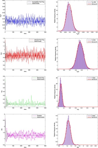
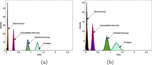
Figure 7. (a) This graph presents the distribution of all species of system (4(4) $\{\begin{array}{l}{\displaystyle \frac{\mathrm{d}{X}_S}{\mathrm{d}t}}={\displaystyle \frac{\mathrm{\Pi }{X}_S}{a+X_S}}-\alpha X_S{X}_I-b{X}_S+{\sigma }_1{X}_S{B}_1\left(t\right),\\ {\displaystyle \frac{\mathrm{d}{X}_I}{\mathrm{d}t}}=\alpha X_S{X}_I-{\displaystyle \frac{\text{β}{X}_{I}Z}{m+\mu X_I+\eta Z}}-c{X}_I+{\sigma }_2{X}_I{B}_2\left(t\right),\\ {\displaystyle \frac{\mathrm{d}Y}{\mathrm{d}t}}=\gamma Y-\delta YZ-dY+{\sigma }_{3}Y{B}_3\left(t\right),\\ {\displaystyle \frac{\mathrm{d}Z}{\mathrm{d}t}}=\delta YZ+{\displaystyle \frac{\text{β}{X}_{I}Z}{m+\mu X_I+\eta Z}}-eZ+{\sigma }_{4}Z{B}_4\left(t\right).\end{array}$(4) ) in one picture with intensity of small noise ${\sigma }_1={\sigma }_2=0.03,{\sigma }_3={\sigma }_4=0.01$ and (b) large noise ${\sigma }_1={\sigma }_2=0.06,{\sigma }_3={\sigma }_4=0.03$.

Data availability statement

Our paper contains numerical experimental results, and values for these experiments are included in the paper. The data is freely available.