A mathematical model for the impact of disinfectants on the control of bacterial diseases

Figures & data

Table 1. Descriptions of variables used in the model system (1(1) $\begin{array}{rl}\frac{\mathrm{d}S}{\mathrm{d}t}& =\mathrm{\Lambda }-\text{β}SI-\eta \frac{B}{L+B}S+\delta R-dS,\\ \frac{\mathrm{d}I}{\mathrm{d}t}& =\text{β}SI+\eta \frac{B}{L+B}S-(\nu +\alpha +d)I,\\ \frac{\mathrm{d}R}{\mathrm{d}t}& =\nu I-(\delta +d)R,\\ \frac{\mathrm{d}B}{\mathrm{d}t}& =sB-s_{0}B+(s_1-s_2\frac{k{C}_h}{M+k{C}_h})I-{\pi }_1{\varphi }_1{C}_{h}B,\\ \frac{\mathrm{d}{C}_h}{\mathrm{d}t}& =\varphi B-{\varphi }_0{C}_h-k{C}_h-{\varphi }_1{C}_{h}B.\end{array}$(1) ).

Variables	Descriptions
S	Number of susceptible human population
I	Number of infected human population
R	Number of recovered human population
B	Density of bacteria present in the environment
$C_h$	Chemical concentration of disinfectants/sanitizer

Figure 1. Schematic diagram of model system (1(1) $\begin{array}{rl}\frac{\mathrm{d}S}{\mathrm{d}t}& =\mathrm{\Lambda }-\text{β}SI-\eta \frac{B}{L+B}S+\delta R-dS,\\ \frac{\mathrm{d}I}{\mathrm{d}t}& =\text{β}SI+\eta \frac{B}{L+B}S-(\nu +\alpha +d)I,\\ \frac{\mathrm{d}R}{\mathrm{d}t}& =\nu I-(\delta +d)R,\\ \frac{\mathrm{d}B}{\mathrm{d}t}& =sB-s_{0}B+(s_1-s_2\frac{k{C}_h}{M+k{C}_h})I-{\pi }_1{\varphi }_1{C}_{h}B,\\ \frac{\mathrm{d}{C}_h}{\mathrm{d}t}& =\varphi B-{\varphi }_0{C}_h-k{C}_h-{\varphi }_1{C}_{h}B.\end{array}$(1) ).

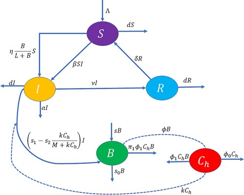
Table 2. Descriptions of parameters involved in system (1(1) $\begin{array}{rl}\frac{\mathrm{d}S}{\mathrm{d}t}& =\mathrm{\Lambda }-\text{β}SI-\eta \frac{B}{L+B}S+\delta R-dS,\\ \frac{\mathrm{d}I}{\mathrm{d}t}& =\text{β}SI+\eta \frac{B}{L+B}S-(\nu +\alpha +d)I,\\ \frac{\mathrm{d}R}{\mathrm{d}t}& =\nu I-(\delta +d)R,\\ \frac{\mathrm{d}B}{\mathrm{d}t}& =sB-s_{0}B+(s_1-s_2\frac{k{C}_h}{M+k{C}_h})I-{\pi }_1{\varphi }_1{C}_{h}B,\\ \frac{\mathrm{d}{C}_h}{\mathrm{d}t}& =\varphi B-{\varphi }_0{C}_h-k{C}_h-{\varphi }_1{C}_{h}B.\end{array}$(1) ).

Parameters	Descriptions
Λ	Rate of immigration into the class of susceptible population
β	Contact rate of susceptibles with infected individuals
η	Transmission rate of susceptible to the infected class due to their
	interaction with bacteria present in the environment
L	Half saturation constant
δ	Rate of transfer of recovered individuals to
	susceptible class due to immunity loss
d	Natural death rate of human population
ν	Recovery rate of human population
α	Disease-induced death rate of human population
s	Self-growth rate of bacteria
$s_0$	Natural death rate of bacteria
$s_1$	Growth rate coefficient of bacteria due to the discharged by infective
	in the environment
$s_2$	Efficacy of chemicals to reduce the density of
	bacteria discharged by infected individuals
k	Per-capita use of chemicals to reduce the density of bacteria
	at source discharged by infected individuals
M	Half saturation constant
${\pi }_1$	Decay coefficient in the density of bacteria present
	in the environment due to the uptake of chemicals
${\varphi }_1$	Per-capita reduction of chemicals due to uptake by bacteria
ϕ	Growth rate of chemicals due to increase in the density of bacteria
${\varphi }_0$	Natural depletion of chemical

Table 3. Values of parameters used for numerical simulations of system (1(1) $\begin{array}{rl}\frac{\mathrm{d}S}{\mathrm{d}t}& =\mathrm{\Lambda }-\text{β}SI-\eta \frac{B}{L+B}S+\delta R-dS,\\ \frac{\mathrm{d}I}{\mathrm{d}t}& =\text{β}SI+\eta \frac{B}{L+B}S-(\nu +\alpha +d)I,\\ \frac{\mathrm{d}R}{\mathrm{d}t}& =\nu I-(\delta +d)R,\\ \frac{\mathrm{d}B}{\mathrm{d}t}& =sB-s_{0}B+(s_1-s_2\frac{k{C}_h}{M+k{C}_h})I-{\pi }_1{\varphi }_1{C}_{h}B,\\ \frac{\mathrm{d}{C}_h}{\mathrm{d}t}& =\varphi B-{\varphi }_0{C}_h-k{C}_h-{\varphi }_1{C}_{h}B.\end{array}$(1) ).

Parameters	Units	Values	References
Λ	persons day${}^{-1}$	5	[29]
β	person${}^{-1}$day${}^{-1}$	0.000004	[29, 45]
η	day${}^{-1}$	0.0005	[36]
L	cells mm${}^{-3}$	1000	[36]
δ	day${}^{-1}$	0.002	Assumed
ν	day${}^{-1}$	0.2	[29, 45]
α	day${}^{-1}$	0.00001	[29, 45]
d	day${}^{-1}$	0.00004	[29, 45]
s	day${}^{-1}$	0.02	[36]
$s_0$	day${}^{-1}$	0.08	[36]
$s_1$	cells mm${}^{-3}$person${}^{-1}$day${}^{-1}$	0.05	[46]
$s_2$	cells mm${}^{-3}$person${}^{-1}$day${}^{-1}$	0.01	Assumed
k	day${}^{-1}$	0.1	Assumed
M	ml day${}^{-1}$	10	Assumed
${\pi }_1$	cells mm${}^{-3}$ ml${}^{-1}$	2	Assumed
${\varphi }_1$	mm${}^3$ cell${}^{-1}$ day${}^{-1}$	0.01	Assumed
ϕ	ml mm${}^3$ cell${}^{-1}$ day${}^{-1}$	0.05	Assumed
${\varphi }_0$	day${}^{-1}$	0.01	Assumed

Figure 2. The normalized forward sensitivity indices of the basic reproduction number (${\mathcal{R}}_0$) with respect to the model parameters Λ, β, η, L, ν, $s_1$, $s_0$ and s. Here, the values of parameters are chosen from Table 3.

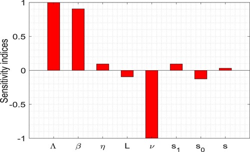
Figure 3. The uncertainty of the model (1(1) $\begin{array}{rl}\frac{\mathrm{d}S}{\mathrm{d}t}& =\mathrm{\Lambda }-\text{β}SI-\eta \frac{B}{L+B}S+\delta R-dS,\\ \frac{\mathrm{d}I}{\mathrm{d}t}& =\text{β}SI+\eta \frac{B}{L+B}S-(\nu +\alpha +d)I,\\ \frac{\mathrm{d}R}{\mathrm{d}t}& =\nu I-(\delta +d)R,\\ \frac{\mathrm{d}B}{\mathrm{d}t}& =sB-s_{0}B+(s_1-s_2\frac{k{C}_h}{M+k{C}_h})I-{\pi }_1{\varphi }_1{C}_{h}B,\\ \frac{\mathrm{d}{C}_h}{\mathrm{d}t}& =\varphi B-{\varphi }_0{C}_h-k{C}_h-{\varphi }_1{C}_{h}B.\end{array}$(1) ) on infected individuals (I). Baseline values of parameters are the same as in Table 3 except $\eta =0.005$. Significant parameters are marked by $\ast$ (p-value $<0.05$).

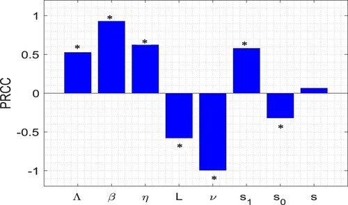
Figure 4. Contour plots of the basic reproduction number (${\mathcal{R}}_0$) as a functions of $s_0-s$ and ν. Rest of the parameters are at the same values as in Table 3. In the figure, dashed green line stands for ${\mathcal{R}}_0=1$. (For interpretation of the references to color in this figure legend, the reader is referred to the web version of this article.)

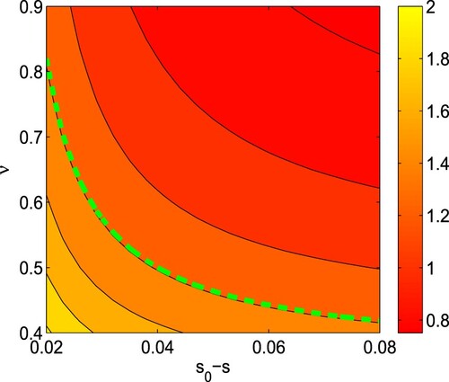
Figure 5. Bifurcation diagram of system (1(1) $\begin{array}{rl}\frac{\mathrm{d}S}{\mathrm{d}t}& =\mathrm{\Lambda }-\text{β}SI-\eta \frac{B}{L+B}S+\delta R-dS,\\ \frac{\mathrm{d}I}{\mathrm{d}t}& =\text{β}SI+\eta \frac{B}{L+B}S-(\nu +\alpha +d)I,\\ \frac{\mathrm{d}R}{\mathrm{d}t}& =\nu I-(\delta +d)R,\\ \frac{\mathrm{d}B}{\mathrm{d}t}& =sB-s_{0}B+(s_1-s_2\frac{k{C}_h}{M+k{C}_h})I-{\pi }_1{\varphi }_1{C}_{h}B,\\ \frac{\mathrm{d}{C}_h}{\mathrm{d}t}& =\varphi B-{\varphi }_0{C}_h-k{C}_h-{\varphi }_1{C}_{h}B.\end{array}$(1) ) with respect to ${\mathcal{R}}_0$. Parameters are at the same values as in Table 3 except $\alpha =0.001$, d = 0.004, $s_2=0.04$ and ${\pi }_1=10$. Here, blue, red and magenta colours, respectively, denote the stable disease-free equilibrium ($E_0$), unstable disease-free equilibrium ($E_0$) and the stable endemic equilibrium ($E^{\ast }$). (For interpretation of the references to color in this figure legend, the reader is referred to the web version of this article.)

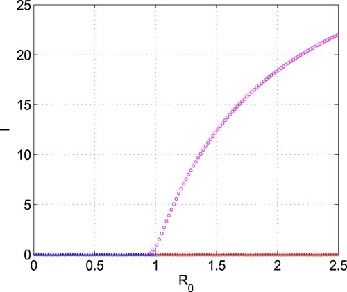
Figure 6. Surface plots of the infective population (first column) and bacterial density (second column) with respect to (a) β and $s_2$, and (b) η and ${\pi }_1$. Other parameters are at the same values as in Table 3.

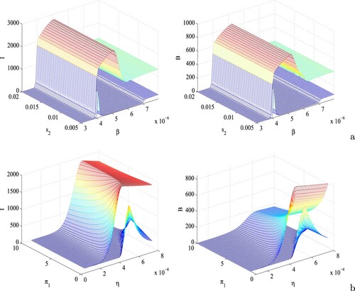
Figure 7. Surface plots of the infective population (first column) and bacterial density (second column) with respect to (a) ϕ and ${\varphi }_0$, and (b) $s_1$ and k. Other parameters are at the same values as in Table 3.

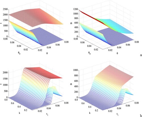
Figure 8. Variations in the infective population (first column) and bacterial density (second column) with respect to time for different combinations of (a) $s_2$ and ${\pi }_1$, and (b) k and ${\varphi }_1$. Rest of the parameters are at the same values as in Table 3 except $\text{β}=0.000003$.

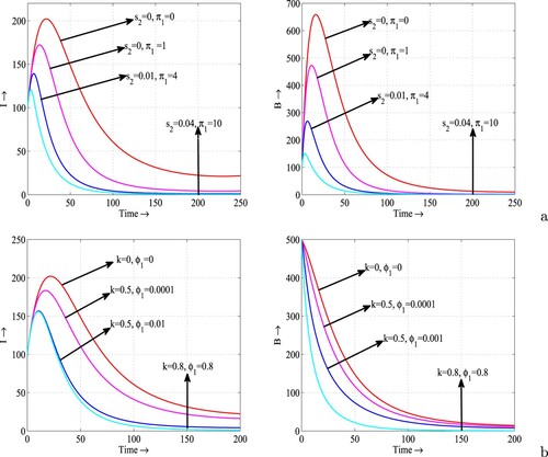
Figure 9. Figure illustrating the global asymptotic stability of disease-free equilibrium $E_0$ in (a) I−R−B and (b) $I-R-C_h$ spaces. Parameters are at the same values as in Table 3 except $\alpha =0.001$, d = 0.004, $s_2=0.04$ and ${\pi }_1=14$. Rest of the parameters are at the same values as in Table 3.

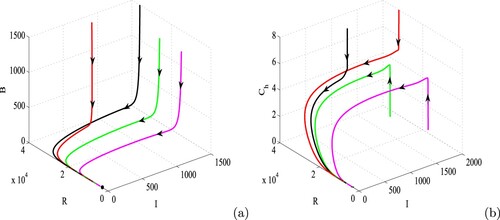
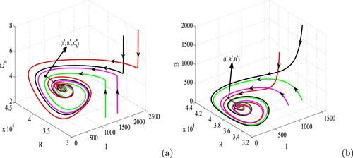
Figure 10. Global stability of the endemic equilibrium $E^{\ast }$ in (a) $I-R-C_h$ (b) I−R−B spaces.

A.K. Misra, R.K. Rai, and Y. Takeuchi, Modeling the control of infectious diseases: Effects of TV and social media advertisements, Math. Biosci. Eng. 15(6) (2018), pp. 1315–1343.

 PubMed Web of Science ®Google Scholar

P.K. Tiwari, R.K. Rai, A.K. Misra, and J. Chattopadhyay, Dynamics of infectious diseases: Local versus global awareness, Int. J. Bifurcat. Chaos 31(07) (2021), pp. 2150102.

 Web of Science ®Google Scholar

R.K. Rai, A.K. Misra, and Y. Takeuchi, Modeling the impact of sanitation and awareness on the spread of infectious diseases, Math. Biosci. Eng. 16(2) (2019), pp. 667–700.

 PubMed Web of Science ®Google Scholar

P.K. Tiwari, R.K. Rai, R.K. Gupta, M. Martcheva, and A.K. Misra, Modeling the control of bacterial disease by social media advertisements: Effects of awareness and sanitation, J. Biol. Syst. 30(01) (2022), pp. 51–92.

 Web of Science ®Google Scholar