Threshold dynamics of a stochastic mathematical model for Wolbachia infections

Figures & data

Figure 1. Extinction of the uninfected mosquitoes. (a) $\theta =0.2$; (b) $\theta =1$. All other parameter values were fixed as: q = 0.2, $\tau =1$, b = 0.02, d = 0.02, D = 0.01, $\theta =0.2$ and initial value $\left(I\right(0),U(0\left)\right)=(0.5,0.5).$

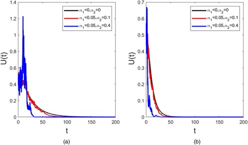
Figure 2. These plots show that sensitivity of $k,{\alpha }_2$ on $R_0$. (a) We set ${\alpha }_2=0.5$ and ${\alpha }_2=0.01$ ; (b) We set k = 0.1 and k = 0.8, and all other parameter values were fixed as: $\tau =0.3$, b = 0.1, q = 0.2.

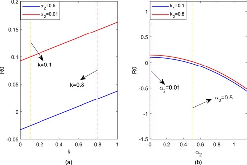
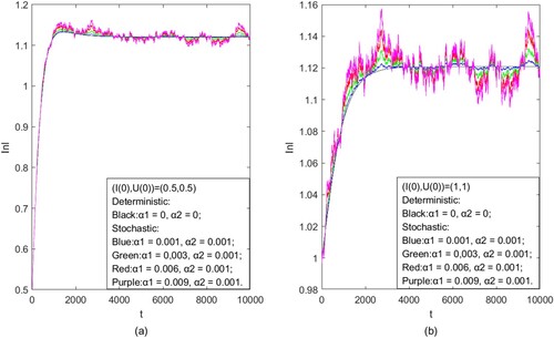
Figure 3. Stationary distribution of deterministic model and stochastic model: (a) we set initial values as $\left(I\right(0),U(0)=(0.5,0.5)$; (b) we set initial values as $\left(I\right(0),U(0)=(1,1)$. The initial values of the solution illustrated by the black line were fixed as $\left(X_1\right(0),X_2(0),Y(0\left)\right)=(10,10,0.5)$, and all other parameters were fixed as: $\tau =0.3$, b = 0.1, d = 0.1, D = 0.01, $\theta =0.2$, q = 0.2, q = 0.3.