Effects of prey refuge and predator cooperation on a predator–prey system

Figures & data

Figure 1. The left and right panels plot components of the unique positive equilibrium and the determinant of $J\left(E^{\ast }\right)$, respectively. Fixed parameter values are $\lambda =10$ and $\text{β}=3$ with c varying between 0 and 0.5. The solid and dashed curves in (a), (c), and (e) denote the x and y components of the positive equilibrium, respectively.

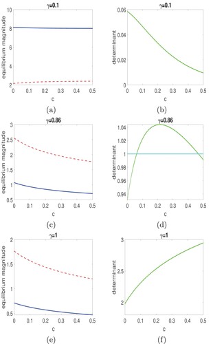
Figure 2. Phase portrait along with the unstable positive equilibrium for system (2(2) $\begin{array}{rl}{x}_{n+1}& =\frac{\lambda (1-\gamma )x_n}{1+x_n}+\frac{\lambda \gamma x_n}{1+x_n}{\mathrm{e}}^{-y_n(1+c{y}_n)},\\ y_{n+1}& =\text{β}\gamma x_n(1-{\mathrm{e}}^{-y_n(1+c{y}_n)}),\\ & x_0,y_0\ge 0.\end{array}$(2) ) are plotted with fixed parameter values of $\lambda =10$, $\gamma =1$, and $\text{β}=0.3$. The degree of hunting cooperation is c = 0.4 in (a) and c = 0.5 in (b). These demonstrate that hunting cooperation destabilizes the predator–prey interaction when there is no prey refuge.

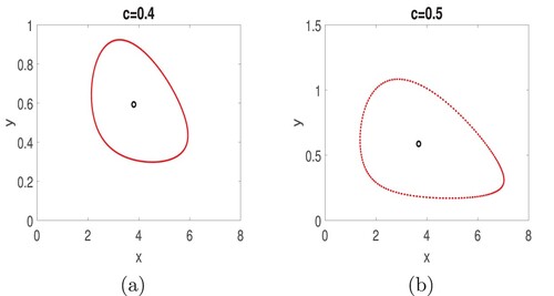
Figure 3. Fixed parameter values are $\lambda =3$, $\text{β}=4$ and $\gamma =0.1$. A bifurcation diagram with respect to c is given in (a) and (b)–(c) present basins of attraction of $E_2^{\ast }$ (in red) and of $E_0$ (in cyan). The degree of hunting cooperation is c = 5 in (b) and c = 8 in (c).

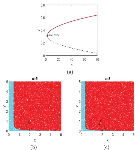
Figure 4. Bifurcation diagrams with respect to c for $0\le c\le 5$ are plotted. Fixed parameter values are $\lambda =10$ and $\text{β}=0.3$. The value of γ is 0.9 in (a)–(b), 0.6 in (c)–(d) and 0.3 in (e)–(f).

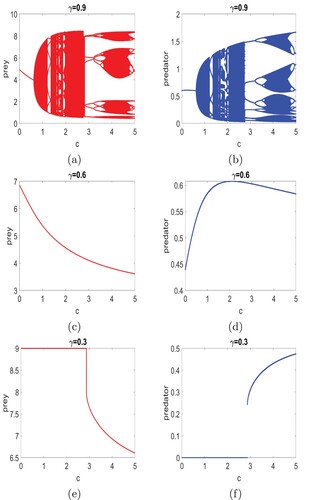
Figure 5. Bifurcation diagrams with respect to γ for $0\le \gamma \le 1$ are plotted. Fixed parameter values are $\lambda =10$ and $\text{β}=0.3$. The parameter value of c is 0 in (a)–(b), 0.9 in (c)–(d), and 25 in (e)–(f).

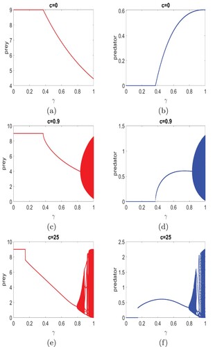
Figure 6. Bifurcation diagrams with respect to β are plotted. Fixed parameter values are $\lambda =2$ and c = 0.2. The other parameter is $\gamma =0.9$ in (a)–(b), $\gamma =0.7$ in (c)–(d), and $\gamma =0.6$ in (e)–(f).

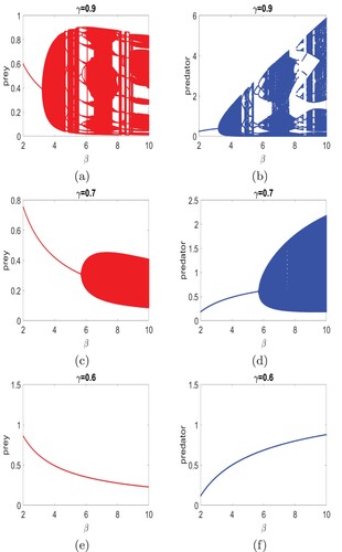
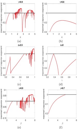
Figure 7. Maximal Lyapunov exponents with respect to c in (a)–(b) and γ in (c)–(d) are approximated. Fixed parameter values are $\lambda =10$ and $\text{β}=0.3$. Plots (e) and (f) present the maximal Lyapunov exponents with respect to β with $\gamma =0.9$ in (e) and $\gamma =0.7$ in (f). The other parameter values are $\lambda =2$ and c = 0.2.