Adaptive delayed reproduction in a 2-dimensional discrete-time competition model

Figures & data

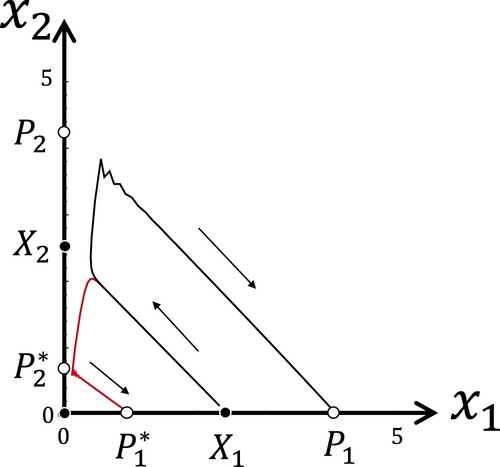
Figure 1. The phase plane $(x_1,x_2)$ of system (1(1) $\{\begin{array}{l}{x}_1(n+1)=x_1(n)\{(1-\eta )\exp (\lambda -x_1(n)-x_2(n))+\eta s\}\\ x_2(n+1)=x_2(n)\exp (\lambda -x_1(n)-x_2(n)),\end{array}$(1) ). The set $D_1$ is a proper subset of $D_2$. Species 1 is dominated by species 2. The unstable manifold of $(X_1,0)$ and the stable manifold of $(0,X_2)$ have nonempty intersections with the interior of ${\mathbb{R}}_{+}^2$.

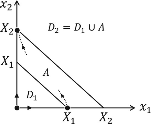
Table 1. Stability of the boundary fixed points and the boundary 2-cycles of system (1(1) $\{\begin{array}{l}{x}_1(n+1)=x_1(n)\{(1-\eta )\exp (\lambda -x_1(n)-x_2(n))+\eta s\}\\ x_2(n+1)=x_2(n)\exp (\lambda -x_1(n)-x_2(n)),\end{array}$(1) ).

	$0<\lambda <2$	$2<\lambda <{\lambda }_2$		${\lambda }_2<\lambda$
		$s<\frac{1}{\cosh \xi }$	$s>\frac{1}{\cosh \xi }$
$(0,0)$	U	U	U	U
$(X_1,0)$	U	U	U	U
$(0,X_2)$	AS	U	U	U
$\{(P_1,0),(P_1^{\ast },0)\}$	–	U	AS	U
$\{(0,P_2),(0,P_2^{\ast })\}$	–	AS	U	U

Note: AS and U stand for asymptotically stable and unstable, respectively.

Figure 2. The parameter plane $(\lambda ,s)$ of system (1(1) $\{\begin{array}{l}{x}_1(n+1)=x_1(n)\{(1-\eta )\exp (\lambda -x_1(n)-x_2(n))+\eta s\}\\ x_2(n+1)=x_2(n)\exp (\lambda -x_1(n)-x_2(n)),\end{array}$(1) ) with $\eta \approx 0$. In regions A, B, and C, $(0,X_2)$, ${\mathcal{P}}_2$, and ${\mathcal{P}}_1$ are asymptotically stable, respectively. There are no stable fixed points nor stable 2-cycles on the boundary of ${\mathbb{R}}_{+}^2$ if $\lambda >{\lambda }_2$.

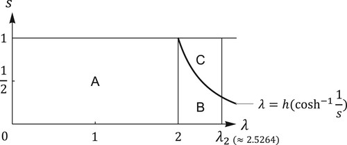
Figure 3. The parameter plane $(\lambda ,s)$ of system (1(1) $\{\begin{array}{l}{x}_1(n+1)=x_1(n)\{(1-\eta )\exp (\lambda -x_1(n)-x_2(n))+\eta s\}\\ x_2(n+1)=x_2(n)\exp (\lambda -x_1(n)-x_2(n)),\end{array}$(1) ). The green and red regions correspond to the region B and C in Figure 2, respectively. In the yellow region, both ${\mathcal{P}}_1$ and ${\mathcal{P}}_2$ have unstable transversal eigenvalues, i.e. both species can mutually invade at the boundary 2-cycles. On the left and right panels, $\eta =0.01$ and $\eta =0.1$, respectively.

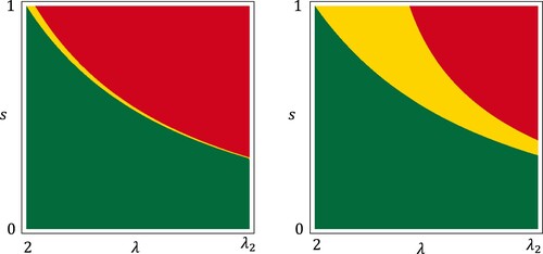
Figure 4. The basins of attraction of the boundary 2-cycles of system (1(1) $\{\begin{array}{l}{x}_1(n+1)=x_1(n)\{(1-\eta )\exp (\lambda -x_1(n)-x_2(n))+\eta s\}\\ x_2(n+1)=x_2(n)\exp (\lambda -x_1(n)-x_2(n)),\end{array}$(1) ). The vertical and horizontal axes are $x_1$ and $x_2$, respectively. (a) The points in the green and yellow regions are attracted by $(P_1,0)$ and $(P_1^{\ast },0)$, respectively, under the second iterate of system (1(1) $\{\begin{array}{l}{x}_1(n+1)=x_1(n)\{(1-\eta )\exp (\lambda -x_1(n)-x_2(n))+\eta s\}\\ x_2(n+1)=x_2(n)\exp (\lambda -x_1(n)-x_2(n)),\end{array}$(1) ). The parameters are $\lambda =2.5$, s = 0.6, and $\eta =0.1$. (b) The points in the black and red regions are attracted by $(0,P_2)$ and $(0,P_2^{\ast })$, respectively, under the second iterate of system (1(1) $\{\begin{array}{l}{x}_1(n+1)=x_1(n)\{(1-\eta )\exp (\lambda -x_1(n)-x_2(n))+\eta s\}\\ x_2(n+1)=x_2(n)\exp (\lambda -x_1(n)-x_2(n)),\end{array}$(1) ). The parameters are $\lambda =2.5$, s = 0.1, and $\eta =0.1$.

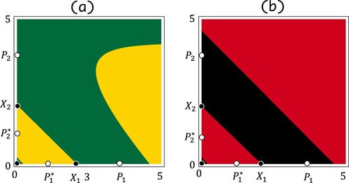
Figure 5. A single forward orbit of system (1(1) $\{\begin{array}{l}{x}_1(n+1)=x_1(n)\{(1-\eta )\exp (\lambda -x_1(n)-x_2(n))+\eta s\}\\ x_2(n+1)=x_2(n)\exp (\lambda -x_1(n)-x_2(n)),\end{array}$(1) ). The points of the orbit are connected with black and red lines if they are points of $2n$th and 2n + 1th iteration, respectively. The parameters are the same as in Figure 4 (a).