
Figures & data
Table 1. Model parameters and their interpretations.
Figure 1. Let the parameters and
be specified as in (Equation10
(10)
(10) ). Then we get
. By selecting
, and plotting the graphs of
and
in panels
and (D), respectively, we obtain the above figure, which illustrates the global attractivity of
.
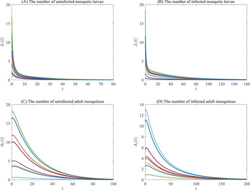
Figure 2. Suppose that the parameters and
in system (Equation1
(1)
(1) ) are in line with (Equation10
(10)
(10) ). Then
. By choosing
, we get the graphs of
and
in panels
and (D), respectively.
![Figure 2. Suppose that the parameters α,d0,μ and d1 in system (Equation1(1) {dJUdt=12βAUAUAU+AI−[d0+d1(JU+JI)]JU−αJU:=f¯1(JU,JI,AU,AI),dJIdt=12βAI−[d0+d1(JU+JI)]JI−αJI:=f¯2(JU,JI,AU,AI),dAUdt=αJU−μAU:=f¯3(JU,JI,AU,AI),dAIdt=αJI−μAI:=f¯4(JU,JI,AU,AI),(1) ) are in line with (Equation10(10) α=0.129,d0=0.05,μ=0.06andd1=0.035.(10) ). Then β∗≈0.1665. By choosing β=0.25>β∗, we get the graphs of JU(t),JI(t),AU(t) and AI(t) in panels (A),(B),(C) and (D), respectively.](/cms/asset/1561def4-3a39-4aa3-ac8b-aac3c114f18a/tjbd_a_2249024_f0002_oc.jpg)
Figure 3. Let the relevant parameters in (Equation2(2)
(2) ) are specified as in Example 3.3. Then the graph of F against x is shown in the above figure, where the left and right red dashed straight lines in the thumbnail represent
and
, respectively, and the intersection point of F and x-axis, marked with asterisk, corresponds to the first component of the unique equilibrium of (Equation2
(2)
(2) ) in Example 3.3.
![Figure 3. Let the relevant parameters in (Equation2(2) {dJUdt=12βAUAUAU+AI−[d0+d1(JU+JI)]JU−αJU−cmJUJU+aP:=f~1(JU,JI,AU,AI,P),dJIdt=12βAI−[d0+d1(JU+JI)]JI−αJI−cmJIJI+aP:=f~2(JU,JI,AU,AI,P),dAUdt=αJU−μAU:=f~3(JU,JI,AU,AI,P),dAIdt=αJI−μAI:=f~4(JU,JI,AU,AI,P),dPdt=mJUJU+aP+mJIJI+aP−δP:=f~5(JU,JI,AU,AI,P),(2) ) are specified as in Example 3.3. Then the graph of F against x is shown in the above figure, where the left and right red dashed straight lines in the thumbnail represent x=aδ2m−δ and x=aδm−δ, respectively, and the intersection point of F and x-axis, marked with asterisk, corresponds to the first component of the unique equilibrium of (Equation2(2) {dJUdt=12βAUAUAU+AI−[d0+d1(JU+JI)]JU−αJU−cmJUJU+aP:=f~1(JU,JI,AU,AI,P),dJIdt=12βAI−[d0+d1(JU+JI)]JI−αJI−cmJIJI+aP:=f~2(JU,JI,AU,AI,P),dAUdt=αJU−μAU:=f~3(JU,JI,AU,AI,P),dAIdt=αJI−μAI:=f~4(JU,JI,AU,AI,P),dPdt=mJUJU+aP+mJIJI+aP−δP:=f~5(JU,JI,AU,AI,P),(2) ) in Example 3.3.](/cms/asset/28947481-e04c-4084-a23c-575492f2a366/tjbd_a_2249024_f0003_oc.jpg)
Figure 4. Assume that the parameters in system (Equation2(2)
(2) ) are defined the same as in Example 3.3. Then the conditions for Theorem 3.4 are satisfied, and there exists six equilibria:
and
. Moreover, equilibria
and
are unstable, equilibria
and
are asymptotically stable.
![Figure 4. Assume that the parameters in system (Equation2(2) {dJUdt=12βAUAUAU+AI−[d0+d1(JU+JI)]JU−αJU−cmJUJU+aP:=f~1(JU,JI,AU,AI,P),dJIdt=12βAI−[d0+d1(JU+JI)]JI−αJI−cmJIJI+aP:=f~2(JU,JI,AU,AI,P),dAUdt=αJU−μAU:=f~3(JU,JI,AU,AI,P),dAIdt=αJI−μAI:=f~4(JU,JI,AU,AI,P),dPdt=mJUJU+aP+mJIJI+aP−δP:=f~5(JU,JI,AU,AI,P),(2) ) are defined the same as in Example 3.3. Then the conditions for Theorem 3.4 are satisfied, and there exists six equilibria: E~0,E~1,E~2,E~3,E~4 and E~∗. Moreover, equilibria E~0,E~1,E~2 and E~∗ are unstable, equilibria E~3 and E~4 are asymptotically stable.](/cms/asset/5664ad7f-f898-4b65-8dda-9c7ddd0519be/tjbd_a_2249024_f0004_oc.jpg)
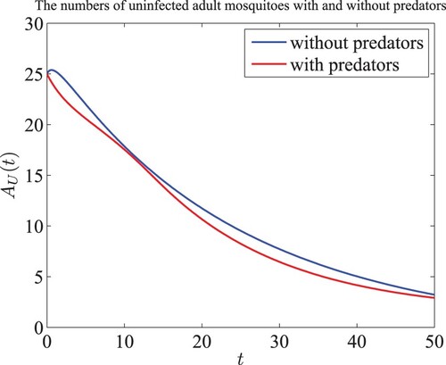
Figure 5. We choose the parameters in Figures C and C and set . Then obtain the numbers of uninfected adult mosquitoes with and without predators.
Data availability statements
Data sharing is not applicable to this article as no new data were created or analysed in this study.