Magnetotelluric signatures of the complex tertiary fold–thrust belt and extensional fault architecture beneath Brøggerhalvøya, Svalbard

Figures & data

Figure 1. (a) The Svalbard Archipilago with its Tertiary affected section along the transform Hornsund Fault Zone (HFZ) highlighted. The map includes locations of Carboniferous basin strata: the Billefjorden Trough adjacent to the Billefjorden Fault Zone (BFZ), the Lomfjorden Fault zone (LFZ), Inner Hornsund Trough (IHT) and St. Jonsfjorden Trough (SJT). Note also the Tertiary Forlandsundet Graben just south of Brøggerhalvøya. The map is modified and redrawn from Bergh et al. (2000) and Saalmann & Thiedig (2002). (b) The MT studied area on Brøggerhalvøya, also represented in (a) and (c) with blue frames. The MT sites are indicated by the black dots and the pink dots denote sites with measured vertical magnetic fields in addition to the horizontal EM components. (c) The red box indicates the surface area of our 3D model.

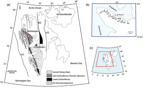
Figure 2. Geoelectric strike and dimensionality. (a) Phase tensor ellipses of the 13 measured sites with their error accounted skew angles (β^∗ ) in colour fills. (b – e) Phase tensor strike estimates for period intervals manifesting a collective dimensionality behaviour. (f) Phase tensor strike estimate for the entire data set (0.003–1000 s). The analysis in general indicates strong 3D effects, with some localized underlying 2D structures and a weak regionally dominant strike direction suitable for the entire data set.

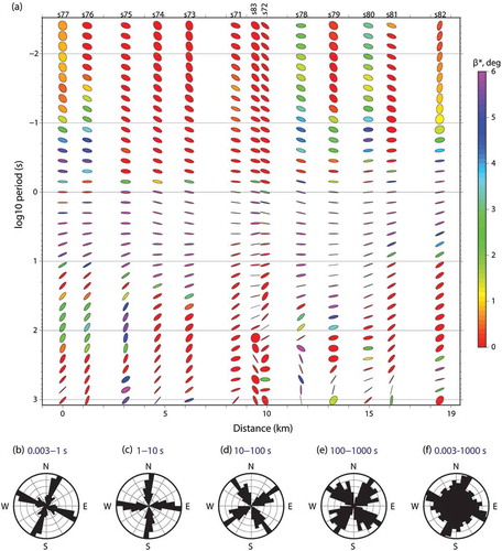
Figure 3. Real part of the induction arrows of the sites s71, s83, s72, s81 and s82 respectively in north-west–south-east direction, in Wiese convention. The arrows are plotted for 1, 8, 64 and 724 seconds in (a) through (d), respectively. The strike directions indicated by the arrows display a reasonable match with the phase tensor strike estimates shown in Fig. 2b–e.

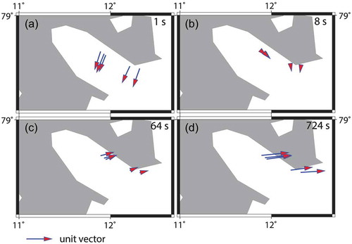
Figure 4. The site by site data misfit between the observed (orange dots) and predicted (black solid lines) determinant data apparent resistivity (Ωm in log10 scale) and phase (deg) parameters underlying the preferred 2D inversion model displayed in Fig. 5b having 1.16 as its overall RMS misfit. All the modelled sites are included in the plot ordered from top – bottom right following the MT profile’s WNW–ESE direction. The y axes are given in log10 scales in seconds.

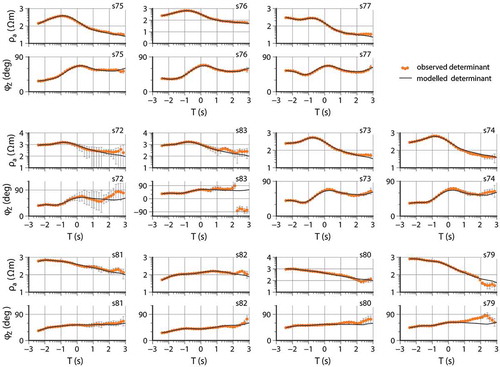
Figure 5. The preferred 2D MT model displayed together with bedrock geology for comparison. (a) A simplified surface geology map for Brøggerhalvøya illustrating the major fold–thrust belt structures and younger, crosscutting normal fault systems; simplified and redrawn from Bergh et al. (2000). (b) The 2D MT model. The MT model anomalies (R, C1 – C4) reasonably correspond with the geology and their interpretation is listed in the colour key in a coinciding manner with the bedrock map. Geological cross-sections that are redrawn from Bergh et al. (2000) are displayed in (c) through (e).

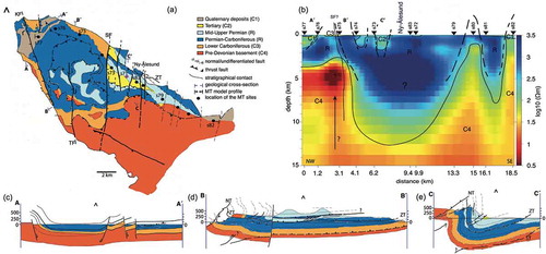
Figure 6. The 3D resistivity model obtained by inverting all the four components of the impedance tensor. The model has an overall misfit RMS 1.68, obtained after 300 iterations. Data fits of the model are displayed site by site with black solid lines in Fig. 8.

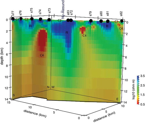
Figure 7. (a) The preferred final 3D model obtained by inverting the full impedance tensor by including detailed bathymetry and the tipper data. The 3D model is supported by the 2D result presented earlier and reflects a geologically meaningful reconstruction of the subsurface bedrock architecture. Interpretation of the model anomalies (R, C1 – C4) can be read from the colour key in Fig. 5. (b) Schematic presentation of the MT final model’s geological and structural interpretation along the studied WNW–ESE profile, showing a horst-graben geometry of alternating, uplifted pre-Devonian unit (C4) and down-faulted Permian–Carboniferous strata (C2 – C3, R).

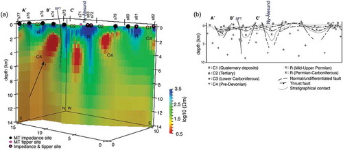
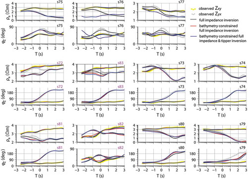
Figure 8. Data misfit between the observed data and results of three different 3D inversion procedures. The misfit is presented site by site for the observed Z_xy (yellow dots) and Z_yx (grey dots) impedance components in measurement coordinate system. The site names in purple represent the sites with the tipper data included in the inversion. For each site the apparent resistivity (Ωm) and the phase (deg) parameters are presented in the top and bottom panels, respectively. The data fit for the model presented in Fig. 6 (full impedance inversion; RMS = 1.68) is denoted with black solid lines, when bathymetry is included in the modelling (RMS = 2.17) in red solid lines and the final model (Fig. 7a, RMS = 2.2) data fits are shown with blue solid lines. The sites are ordered from top left to bottom right matching the MT profile’s WNW–ESE direction and in the same order as in Fig. 4.

Bergh S.G., Maher H.D. & Braathen A. 2000. Tertiary divergent thrust directions from partitioned transpression, Brøggerhalvøya, Spitsbergen. Norwegian Journal of Geology 80, 63–81.

 Google Scholar

Saalmann K. & Thiedig F. 2002. Thrust tectonics on Brøggerhalvøya and their relationship to the Tertiary West Spitsbergen Fold-and-Thrust Belt. Geological Magazine 139, 47–72.

 Web of Science ®Google Scholar