Global land mapping of satellite-observed CO₂ total columns using spatio-temporal geostatistics

Figures & data

Figure 1. Example of the spatial distribution and variation of the used ACOS-GOSAT XCO₂ retrievals for four months of (a) July 2009, (b) October 2009, (c) January 2010 and (d) April 2010 over global land.

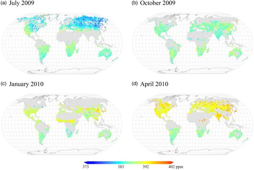
Figure 2. (a) Global spatial distribution density of the used ACOS-GOSAT XCO₂ retrievals (after filtering) from June 2009 to May 2013 in terms of available data number in grids of 5°longitude by 5°latitude and (b) temporal variation of available ACOS-GOSAT retrievals (after filtering) in each 3-day interval. The dashed rectangle area in (a) from 5 to 15°N and 20°W to 40°E covers the tropical region in central Africa, which will be used in Sections 4.5 and 4.6.

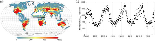
Table 1. Annual statistics for the ACOS-GOSAT v3.3 XCO₂ global land data used in this study after filtering and bias-correction.

	Number of retrievals	Minimum (ppm)	Maximum (ppm)	Mean (ppm)	Standard deviation (ppm)
June 2009–May 2010	58,437	355.89	403.65	386.73	3.11
June 2010–May 2011	67,840	375.72	406.60	389.01	2.92
June 2011–May 2012	67,987	357.58	404.66	390.73	2.94
June 2012–May 2013	65,360	378.92	408.14	392.82	2.95

Figure 3. Global distribution of the 16 TCCON sites used for the comparison with the mapping dataset, and the global land study area for mapping in gray.

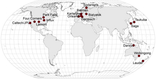
Figure 4. NOAA Earth System Research Laboratory (ESRL) annual mean global CO₂ growth rate for the year 2000 to 2013, published in ESRL-NOAA webpage: http://www.esrl.noaa.gov/gmd/ccgg/trends/global.html.

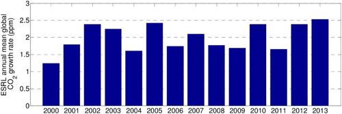
Figure 5. Workflow chart for the spatio-temporal mapping process and the evaluation of the mapping data products in this study. The input datasets are displayed in bold and the numbers in the boxes denote the section numbers in the manuscript.

Figure 6. (a) Overview of the global spatio-temporal distribution of XCO₂ as a function of latitude and time from original ACOS-GOSAT data aggregated with a grid resolution of 5° in latitude and one month in time and (b) the corresponding deterministic spatio-temporal trend calculated from model simulation of CarbonTracker CT2013 XCO₂ data with a grid resolution of 2° in latitude and one time-unit (3-day) in time.

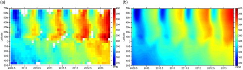
Table 2. Zonal statistics for the 11 bands, including the central latitude of each 10° latitude zone, the number of available data, the median and standard deviation of the ACOS-GOSAT XCO₂ data from June 2009 to May 2013 in the corresponding zone, the parameters of the spatio-temporal variogram model of the ACOS-GOSAT data, and the corresponding nugget/sill ratios in space and time, respectively.

	Zone center latitude	Number of data	Median (ppm)	Standard deviation (ppm)	Estimated parameters for variogram model [, , , , , ]	Spatial ratio nugget/sill	Temporal ratio nugget/sill
Zone 1	65°N	10,462	387.76	4.73	[1.84 ± 0.02, 170.73 ± 4.15, 3.82 ± 0.04, 13.08 ± 0.22, 0.26 ± 0.00, 1.22 ± 0.02]	0.40 ± 0.01	0.24 ± 0.00
Zone 2	55°N	16,461	389.02	4.59	[1.43 ± 0.01, 238.22 ± 3.49, 2.44 ± 0.02, 14.70 ± 0.14, 0.27 ± 0.00, 1.28 ± 0.01]	0.47 ± 0.00	0.34 ± 0.00
Zone 3	45°N	49,821	389.88	4.20	[1.35 ± 0.01, 319.44 ± 4.91, 1.84 ± 0.01, 13.26 ± 0.13, 0.34 ± 0.00, 1.30 ± 0.01]	0.49 ± 0.00	0.41 ± 0.00
Zone 4	35°N	44,095	390.65	3.82	[1.31 ± 0.01, 261.64 ± 6.97, 2.04 ± 0.01, 16.31 ± 0.19, 0.41 ± 0.00, 1.21 ± 0.01]	0.48 ± 0.00	0.37 ± 0.00
Zone 5	25°N	18,374	391.23	3.58	[1.13 ± 0.01, 167.18 ± 4.65, 3.16 ± 0.05, 42.15 ± 0.92, 0.32 ± 0.00, 1.03 ± 0.01]	0.48 ± 0.00	0.25 ± 0.00
Zone 6	15°N	8571	391.82	3.68	[1.44 ± 0.01, 172.63 ± 4.04, 2.75 ± 0.14, 20.82 ± 1.53, 0.32 ± 0.00, 0.87 ± 0.01]	0.38 ± 0.00	0.24 ± 0.01
Zone 7	5°N	2774	391.81	3.57	[2.38 ± 0.07, 384.00 ± 19.16, 2.36 ± 0.21, 17.02 ± 2.31, 0.38 ± 0.01, 0.62 ± 0.02]	0.21 ± 0.01	0.21 ± 0.01
Zone 8	5°S	6678	390.22	2.67	[1.24 ± 0.01, 397.80 ± 5.41, 1.37 ± 0.04, 23.60 ± 0.97, 0.63 ± 0.00, 0.74 ± 0.00]	0.37 ± 0.00	0.35 ± 0.01
Zone 9	15°S	31,771	389.77	2.69	[0.91 ± 0.00, 235.32 ± 2.58, 1.14 ± 0.02, 15.57 ± 0.46, 0.79 ± 0.00, 0.70 ± 0.00]	0.43 ± 0.00	0.38 ± 0.00
Zone 10	25°S	44,436	389.38	2.73	[0.90 ± 0.00, 184.73 ± 1.74, 1.21 ± 0.03, 17.04 ± 0.56, 0.78 ± 0.00, 0.66 ± 0.00]	0.43 ± 0.00	0.35 ± 0.00
Zone 11	35°S	20,754	389.05	2.78	[0.98 ± 0.01, 129.41 ± 2.17, 1.34 ± 0.02, 18.35 ± 0.53, 0.69 ± 0.00, 0.58 ± 0.01]	0.37 ± 0.00	0.30 ± 0.00

Notes: Uncertainties of the variogram-related parameters, quantified by one standard deviation, are derived from the Monte Carlo study described in Section 3.3.

Figure 7. For each latitude zone, the left plot shows the spatio-temporal empirical variogram of the ACOS-GOSAT XCO₂ residual data after the spatio-temporal trend is excluded, and the right plot shows its fitted variogram model using the product-sum model in Equation (4).

Table 3. Summary statistics for the developed spatio-temporal method and spatial-only method from global land cross-validation based on the Monte Carlo sampling technique, including correlation coefficient (r²), MAPE, RMSE, and percentage of prediction error within 1 ppm (PPE1) for the global mapping approach.

r^2	MAPE (ppm)	RMSE (ppm)	PPE1 (%)
Spatio-temporal method
0.94 ± 0.00	0.93 ± 0.01	1.28 ± 0.01	65.53 ± 0.42
Spatial-only method
0.92 ± 0.00	1.06 ± 0.01	1.41 ± 0.01	58.62 ± 0.43

Note: Both mean and one standard deviation of the ensemble outputs from cross-validation are shown.

Figure 8. Temporal variation comparison for the 16 TCCON sites. As shown in these panels, the original ACOS-GOSAT XCO₂ retrievals within 500 km of the TCCON site are in gray dots, the corresponding medians are in black dots when at least three data points are available within the time-unit. The TCCON data, smoothed by applying the ACOS-GOSAT averaging kernel, are indicated by blue circles. The data are chosen using coincidence criteria of within ±2 hours of GOSAT overpass time, and a 3-day (one time-unit) median is calculated for the comparison if the number of data points within the time-unit is at least 3. The predicted TCCON site XCO₂ time series using the global land mapping approach are indicated by the red line.

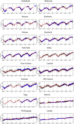
Figure 9. Statistics of comparison between the geostatistical mapping results and the TCCON data (smoothed by applying the ACOS-GOSAT averaging kernel), and between the ACOS-GOSAT 3-day median XCO₂ data and TCCON data, hereafter referred to as Mapping-TCCON and ACOS-TCCON, respectively. The statistics are also shown in Table 4. The top panel shows the comparison of XCO₂ biases between Mapping-TCCON and ACOS-TCCON, while the down panel shows the comparison of numbers of coincident data pairs between them.

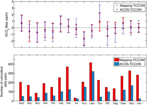
Table 4. Statistics of comparison between the geostatistical mapping results and the TCCON data (smoothed by applying the ACOS-GOSAT averaging kernel), and between the ACOS-GOSAT 3-day median XCO₂ data and TCCON data, hereafter referred to as Mapping-TCCON and ACOS-TCCON, respectively.

		Mapping-TCCON				ACOS-TCCON
Sites	Location [longitude, latitude]	Coincident data pairs	Averaged biases (ppm)	Averaged absolute bias (ppm)	Standard deviation (ppm)	Coincident data pairs	Averaged biases (ppm)	Averaged absolute bias (ppm)	Standard deviation (ppm)
Sodankylä	[26.63, 67.37]	204	0.72	1.05	1.22	50	0.62	1.18	1.22
Bialystok	[23.03, 53.23]	171	−0.56	1.30	1.58	47	−0.47	0.77	0.96
Bremen	[8.85, 53.10]	86	−0.72	1.28	1.51	38	−0.76	1.17	1.43
Karlsruhe	[8.44, 49.10]	190	−0.30	0.97	1.17	86	−0.52	1.09	1.42
Orleans	[2.11, 47.97]	150	−0.47	0.97	1.10	56	−0.72	1.28	1.45
Garmisch	[11.06, 47.48]	253	0.57	1.02	1.14	100	0.56	1.09	1.26
Park Falls	[−90.27, 45.94]	371	0.22	0.78	0.97	123	0.30	0.82	1.05
Influx	[−86.00, 39.86]	32	−0.26	0.63	0.76	23	−0.04	1.02	1.42
FourCorners	[−108.48, 36.80]	206	−1.62	1.68	1.05	151	−1.72	1.72	1.00
Lamont	[−97.49, 36.60]	416	−0.41	0.79	0.90	320	−0.60	0.91	1.00
Tsukuba	[140.12, 36.05]	225	0.86	1.29	1.37	43	2.24	2.24	1.24
JPL/Caltech	[−118.18, 34.20]	148	−0.21	0.90	1.11	99	−1.19	1.58	1.44
Saga	[130.29, 33.24]	135	−0.01	0.67	0.83	12	−0.86	1.21	1.39
Darwin	[130.89, −12.43]	270	0.69	0.91	0.84	118	−0.10	0.66	0.85
Wollongong	[150.88, −34.41]	327	0.14	0.76	0.91	167	−0.00	0.88	1.11
Lauder	[169.68, −45.05]	281	−0.01	0.53	0.66	23	0.16	0.71	0.92
Overall		3465	−0.01	0.94	1.22	1456	−0.35	1.10	1.38

Notes: The statistics include the location information, and statisics of the differences computed by subtracting the TCCON median XCO₂ from the mapping predictions and ACOS-GOSAT XCO₂ 3-day medians, respectively, at the corresponding TCCON sites.

Figure 10. Spatial distribution of seasonal mean XCO₂ from global land mapping for three years of 2010 in panel (a), 2011 in panel (b) and 2012 in panel (c). Four images in each panel corresponds to spring, summer, autumn and winter from left to right, respectively. These global land mapping seasonally averaged results in 1° by 1° grid are obtained by calculating the seasonal mean from the geostatistical mapping results when at least one data is available for each of the three months in that season. As usual, the season spring includes three months of March, April and May, summer includes June, July and August, autumn includes September, October and November, and winter includes December, next year January and February.

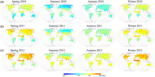
Figure 11. Kriging standard deviations of prediction, a measurement of prediction uncertainty. (a) Spatial distribution, which is obtained by averaging the kriging standard deviations over all time-units in the global land. (b) Temporal distribution for the 11 zones, which are averaged for each time-unit of each zone from June 2009 to May 2013. For each time-unit and each zone, the averages are calculated only when more than 50% of the data are available.

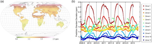
Figure 12. Overview of the global spatio-temporal distribution of XCO₂ as a function of latitude and time, from (a) global land mapping dataset with a grid resolution of 1° in latitude and one time-unit in time, (b) original ACOS-GOSAT data with a grid resolution of 5° in latitude and one month in time, and model simulations from both (c) CarbonTracker CT2013 data with a grid resolution of 2° in latitude and one time-unit in time and (d) GEOS-Chem data in 2010 with a grid resolution of 4° in latitude and one time-unit in time, and an overview of the differences of global spatio-temporal distribution of XCO₂ between (e) global land mapping dataset and CarbonTracker2013 data, (f) global land mapping dataset and GEOS-Chem data, (g) original ACOS-GOSAT data and CarbonTracker CT2013 data, and (h) original ACOS-GOSAT data and GEOS-Chem data.

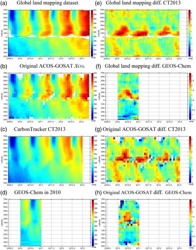
Figure 13. The panel shows the XCO₂ time series in central Africa within 5°N to 15°N in latitude and 20°W to 40°E in longitude. The original ACOS-GOSAT data indicated by gray dots and its mean in black dots calculated when at least three data points are available within the time-unit. The mapping dataset mean is indicated by the blue line, CarbonTracker CT2013 data mean by the red line and GEOS-Chem data mean by the green line.

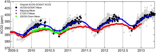
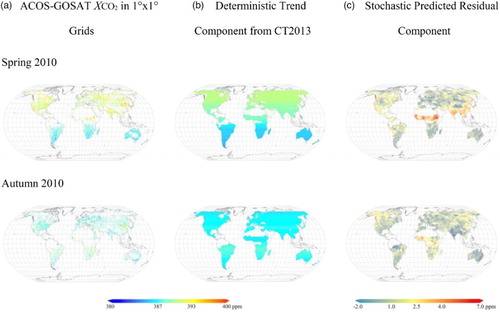
Figure 14. (a) Original ACOS-GOSAT XCO₂ distributions averaged over 1°×1° grids, and the corresponding mapping decompositions, including (b) averaged deterministic trend component from CT2013 and (c) averaged stochastic residual component for Spring 2010 and Autumn 2010, respectively.