Spectral matching techniques (SMTs) and automated cropland classification algorithms (ACCAs) for mapping croplands of Australia using MODIS 250-m time-series (2000–2015) data

Figures & data

Table 1. Ground data samples over Australia for the year 2014.

Code	Crop description	Samples for training	Samples for testing	Samples for an independent accuracy assessment	Samples total number
		N1	N2	N3	N
#	Name	#	#	#	#
1	Alfafa	4	3	4	11
2	Barley	154	153	154	461
3	Beans	30	29	29	88
4	Canola	186	185	186	557
5	Lentils	65	65	65	195
6	Lupin	34	33	35	102
7	Oats	73	72	73	218
8	Peas	27	26	26	79
9	Wheat	283	283	284	850
10	Orchards	55	60	54	169
11	Sown-pasture	95	98	96	289
12	Land prepared for Season 2	20	16	18	54
13	Crop-harvested	9	9	10	28
14	Vegetables	1	1	1	3
15	Plantation	4	3	3	10
16	Cropland,others	30	29	25	84
20	Grazing/pastures	118	117	117	352
30	Non-croplands	145	165	155	465
40	Fallow	125	141	130	396
	Total	1458	1488	1465	4411

Note: The ground data samples were randomly split into: reference or training (N = 1458 samples), validation set 1 for testing accuracies (N = 1488), independent validation set 2 for testing accuracies (N = 1465).

Figure 1. Methodology overview. Methodology workflow showing the integrated analysis of MODIS-NDVI time-series data using QSMTs and ACCA.

Figure 2. Three cropland masks of Australia and the development of ideal spectral signatures (ISSs) for each of these masks. Development of the three cropland masks is defined in Section 3.1. Using precise ground data and MODIS 250 m time-series data, unique and distinctly separable ISSs of the three masks were a total of 13 classes: (a) 4 for the rainfed mask, (b) 3 for the pasture mask, and (c) 6 for the irrigated-mask. The cropland fallow signature was common across. The total 13 classes can be combined to 6 unique classes by combining similar classes across masks.

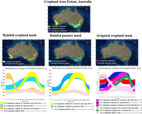
Figure 3. Ideal spectral library of crops. Illustration of few ground data samples collected throughout Australia and their t time-series MODIS 250 m NDVI ideal spectra profiles.

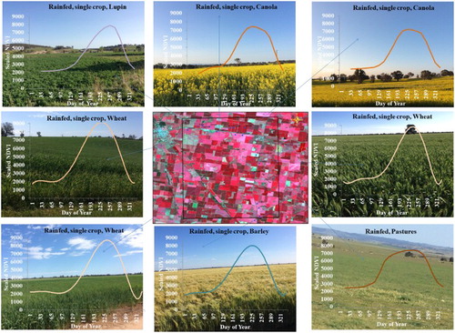
Figure 4. Illustration of SCS R², a QSMT method, to group, match, assess, identify, and label classes. (a) Class spectra: group similar class spectra (e.g. class #’s 3,6,7, 9, … .,41, 44; total 27 similar classes from rainfed mask classification) obtained from ISOCLASS clustering classification, (b) ideal spectra: obtain an ideal spectra from the spectral library that closely matches with the grouped class spectra, (c) class spectra (Figure 4(a)) matched with ideal spectra (Figure 4(b)) using SCS R² values (SCS R² values varied between 0.83 and 0.994, with 26 of 27classes having SCS R-square values of 0.9 or greater), and (d) group of class spectra matched with ideal spectra: combine all similar class spectra into one group and match with ideal spectra which resulted in an SCS R² value of 0.96 leading to labeling of the class spectral classes as similar name as ideal spectral label. So, the class name in this example is: croplands, rainfed, single crop (Season 1), all crops or mixed crops.

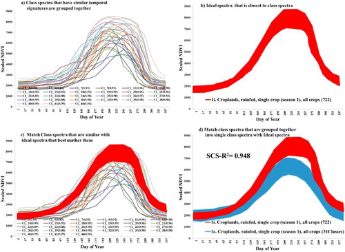
Table 2. SCS R² values, a QSMT, matching class spectra with ideal spectra.

		Class spectra
Ideal spectra		1c	2c	3c	4c	5c	6c
	1i	0.948
	2i		0.977
	3i			0.993
	4i				0.993
	5i					0.883
	6i						0.99

Note: (a) 1i, 2i, 3i, 4i, 5i, and 6i represent ideal spectra developed from ground data and

(b) 1c, 2c, 3c, 4c, 5c, and 6c represent class spectra obtained from unsupervised classification.

Figure 5. An automated cropland classification algorithm (ACCA) for Australia that can be used to compute six cropland classes as well as croplands versus non-croplands year-after-year automatically and accurately.

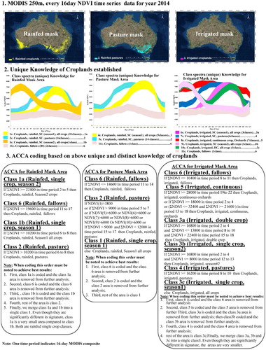
Figure 6. RCP of the year 2014 (RCP2014) for Australia at 250 m.

Note: 1. Total area of cropland (with pasture): 58.55 Mha, total area of cropland (without pasture): 30.80 Mha; 2. the % within brackets in the legend classes are as % of 58.55 Mha.

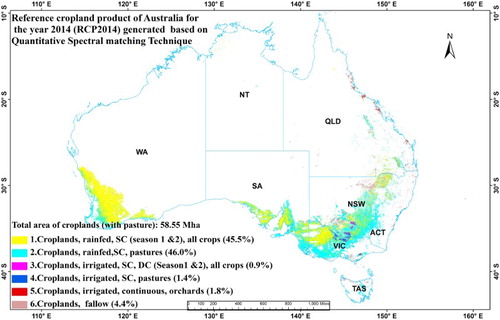
Table 3. Cropland areas of Australia for the year 2014 showing the net cropland areas (without considering cropland intensity) and annualized cropland areas (considering cropland intensity).

	Net Area Season1 (NAS1)			Net Area Season2 (NAS2)			Net Area Continuous (NAC)			Annualized Area (AA) = NAS1 + NAS2 + NAC
	FPA^a	CAF^b	SPA^c	FPA^a	CAF^b	SPA^c	FPA^a	CAF^b	SPA^c	Season 1 + Season 2 +  Continous	Percent of total cropland + pasture area	Percent of total cropland area
Class name	Mha	%	Mha	Mha	%	Mha	Mha	%	Mha	Mha	%	%
1. Croplands, rainfed, SC (Seasons 1 and 2), all crops	28.12	93.2	26.21	0.472	97.6	0.46	N/A	N/A	N/A	26.67	45.5	86.6
2. Croplands, rainfed, SC, pastures	28.34	95.0	26.91	N/A	N/A	N/A	N/A	N/A	N/A	26.91	46.0
3. Croplands, irrigated, SC, DC (Seasons 1 and 2), all crops	0.46	90.3	0.42	0.106	98.6	0.10	N/A	N/A	N/A	0.52	0.9	1.7
4. Croplands, irrigated, SC, pastures	0.85	99.0	0.84	N/A	N/A	N/A	N/A	N/A	N/A	0.84	1.4
5. Croplands, irrigated, continuous, orchards	N/A	N/A	N/A	N/A	N/A	N/A	1.12	94.8	1.06	1.06	1.8	3.4
6. Croplands, fallow^d	2.55	100	2.55							2.55	4.4	8.3
							Total 1: 1–6 (Mha)			58.55	100.00
							Total 2: 1, 3, 5, 6 (Mha)			30.80		100.00

Note: The areas also show cropland with and without pasture. SC = single crop: DC = double crop.

^aFPA (Full pixel area) is determined by reprojecting geographic projection to GDA 1994 Albers projection for Australia.

^bCAF (Crop area fraction) is determined by developing relationship between average NDVI of growing season with percent cover based on literature.

^cSPA(Sub pixel area) = FPA × CAF.

^dCAF for fallow fraction area (FFA) = 100.

Table 4. Accuracy error matrix of the RCP of Australia for the year 2014 (RCP2014 on Y-axis) based on validation ground dataset #1 obtained during field visit (X-axis) also conducted during the year 2014.

		Ground reference data
		1. Croplands, rainfed, all crops	2. Croplands, rainfed, pastures	3. Croplands, irrigated, all crops	4. Croplands, irrigated, Pastures	5. Croplands, irrigated, continuous, orchards	6. Croplands, fallow	7. Non-croplands	Row total (SMT Classified)	Commission error^s
RCP2014	1. Croplands, rainfed, all crops	700	42	0	0	1	0	17	760	5.7%
	2. Croplands, rainfed, pastures	133	101	0	0	5	0	18	257	53.7%
	3. Croplands, irrigated, all crops	0	0	54	2	0	0	0	56	3.6%
	4. Croplands, irrigated, pastures	0	0	9	60	0	0	0	69	13.0%
	5. Croplands, irrigated, continuous, Orchards	0	0	1	1	58	0	7	67	3.0%
	6. Croplands, fallow	2	1	0	0	0	140	0	143	2.1%
	7. Non-croplands	4	8	0	0	0	1	123	136	9.6%
	Column total (ground reference data)	839	152	64	63	64	141	165	1488
	Omission error^b	16.6%	33.6%	15.6%	4.8%	9.4%	0.7%	25.5%
	Producer accuracy^c	83.4%	66.4%	84.4%	95.2%	90.6%	99.3%	74.5%
	User accuracy^d	92.1%	39.3%	96.4%	87.0%	86.6%	97.9%	90.4%
	Over all accuracy^e									83.1%
									Kappa^f	0.747

^aCommission error : pixels that belong to another class but labeled as this class.

^bOmission error: pixels that belong to this class, but are labeled to another class.

^cProducer accuracy: as a producer, 83.4% of the cropland pixels of class 1 in ground reference data were correctly classified as cropland pixels of class 1 in RCP2014.

^dUser accuracy: as a user, 92.1% of the pixels classified as croplands pixels of class 1by RCP2014 were indeed croplands.

^eOverall accuracy = total classification accuracy.

^fKappa value compares observed accuracy (overall) with expected accuracy (random chance).

Table 5. Accuracy Error matrix for the RCP for the year 2014 (RCP2014) conducted by external independent evaluation team based on validation dataset #2 obtained during field visit of year 2014.

	Ground reference data
		1. Cropland	2. Non-cropland	Row total	Commission error^a
RCP 2014	1.Cropland	102	13	115	11.3%
	2. Non-cropland	4	810	814	0.5%
	Column total	106	823	929
	Omission error^b	3.8%	1.6%
	Producer accuracy^c	96.2%	98.4%
	User accuracy^d	88.7%	99.5%
	Overall accuracy^e				98.2%
				Kappa^f	0.91

^aCommission error : pixels that belong to another class but labeled as this class.

^bOmission error : pixels that belong to this class, but are labelled to another class.

^cProducer accuracy: 96.2% of the cropland pixels of class 1 in ground reference data were correctly classified as cropland pixels of Class 1 in RCP2014.

^dUser accuracy: 88.7% of the pixels classified as croplands pixels of class 1by RCP2014 were indeed croplands.

^eOverall accuracy = total classification accuracy.

^fkappa value compares observed accuracy (overall) with expected accuracy (random chance).

Figure 7. ACCA algorithm derived cropland product for the year 2014 (ACP2014) for Australia at 250 m.

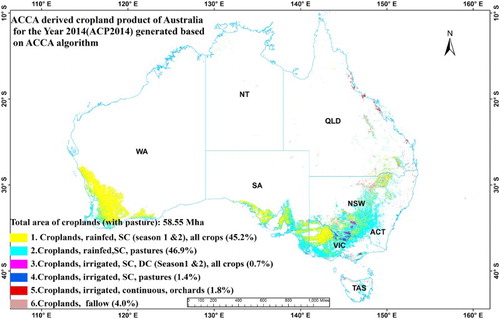
Table 6. Comparison of the statistics from RCP2014 with ACP2014.

Class description	RCP 2014^a	Percent of croplands	ACP 2014^b	Percent of croplands	Percent of ACP2014^b to RCP2014^a
Name	#Pixels	%	#Pixels	%	%
1. Croplands, rainfed, all crops	620,5071	45.5	6,170,793	45.2	99.4
2. Croplands, rainfed, pastures	6,363,457	46.6	6,400,516	46.9	100.6
3. Croplands, irrigated, all crops	105,109	0.8	95,748	0.7	91.1
4. Croplands, irrigated, pastures	189,325	1.4	191,920	1.4	101.4
5. Croplands, irrigated, continuous	237,235	1.7	243,680	1.8	102.7
6. Croplands, fallow	550,761	4.0	548,301	4.0	99.6
Total croplands	13,650,958	100.0	13,650,958	100.0

Note: The statistics of the reference cropland products of the year 2014 (RCP2014) were compared with the statistics of the ACCA-derived cropland product of the year 2014 (ACP2014).

^aReference cropland product for the year 2014 (RCP2014) was produced using QSMTs.

^bAutomated cropland classification algorithm (ACCA) derived cropland product for the year 2014 (ACP 2014) is produced using ACCA algorithm.

Figure 8. ACP2014 versus FAO state by state statistics for irrigated cropland areas of Australia.

Table 7. ACP2014 versus RCP2014 error/similarity matrix.

		RCP2014
		1. Croplands, rainfed, all crops	2. Croplands, rainfed, pastures	3. Croplands, irrigated, all crops	4. Croplands, irrigated, pastures	5. Croplands, irrigated, continuous	6. Croplands, fallow	Row total SMT classified	Commission error^a
ACP2014	1. Croplands, rainfed, all crops	556,5497	621,112	0	0	0	18,462	6,205,071	10.3%
	2. Croplands, rainfed, pastures	520,562	575,3513	0	0	0	89,382	6,363,457	9.6%
	3. Croplands, irrigated, all crops	0	0	75,551	14647	9723	5188	105,109	28.1%
	4. Croplands, irrigated, pastures	0	0	8927	157,372	23,026	0	189,325	16.9%
	5. Croplands, irrigated, continuous, Orchards	0	0	6901	19,849	210,242	243	237,235	11.4%
	6. Croplands, fallow	84,734	25891	4369	52	689	435,026	550,761	21.0%
	Column total (ACCA classified)	6,170,793	6,400,516	95,748	191,920	243,680	548,301	13,650,958
	Omission error^b	9.8%	10.1%	21.1%	18.0%	13.7%	20.7%
	Producer accuracy^c	89.7%	90.4%	71.9%	83.1%	88.6%	79.0%
	User accuracy^d	90.2%	89.9%	78.9%	82.0%	86.3%	79.3%
	Overall accuracy^e								89.4%
								Kappa^f	0.814

Note: Error/similarity matrix comparing ACCA generated cropland product for the year 2014 (ACP2014) with reference cropland product for the year 2014 (RCP2014).

^aCommission error:pixels that belong to another class but labeled as this class.

^bOmission error pixels that belong to this class, but are labelled to another class.

^cProducer accuracy:89.7% of the cropland pixels of class 1 in RCP2014 (reference product) were correctly classified as cropland pixels of Class 1 in ACP2014 (ACCA-derived product).

^dUser accuracy: 90.2% of the pixels classified as croplands pixels of class 1 (by ACCA algorithm) were indeed croplands.

^eOverall accuracy = total classification accuracy.

^fKappa value compares observed accuracy (overall) with expected accuracy (random chance).

Table 8. ACP2014 versus GRIPC500 m (Salmon et al. 2015) accuracy assessment.

	GRIPC^g
		1. Cropland	2. Non-cropland	Row total	Commission error^a
ACP 2014	1. Cropland	10051903	3665084	13716987	26.7%
	2. Non-cropland	2157017	141845510	144002527	1.5%
	Column total	12208920	145510594	157719514
	Omission error^b	17.7%	2.5%
	Producer accuracy^c	82.3%	97.5%
	User accuracy^d	73.3%	98.5%
	Overall accuracy^e				96.3%
				Kappa^f	0.755

Note: Accuracy of ACCA generated cropland product for the year 2014 (ACP2014) versus GRIPC500 m (Salmon et al. 2015).

^aCommission error: pixels that belong to another class but labeled as this class.

^bOmission error: pixels that belong to this class, but are labeled to another class.

^cProducer accuracy: as a producer, 82.3% of the cropland pixels in GRIPC were correctly classified as cropland pixels in ACP2014 (ACCA algorithm derived product).

^dUser accuracy: as a user, 73.3% of the pixels classified as croplands pixels (by ACCA algorithm) were indeed croplands.

^eOverall accuracy = total classification accuracy.

^fKappa value compares observed accuracy (overall) with expected accuracy (random chance).

^gGRIPC = global rainfed and irrigated cropland map at 500 m resolution produced by Salmon et al. (2015).

Table 9. Comparison of Australia’s irrigated areas from different studies.

State	Area equipped for irrigation^a (ha)	Area actually irrigated FAO AQUASTAT^b (ha)	Australia National Statistics (ANS)^c (ha)	GCEV2^d This Study (ha)	GRIPC^e (ha)	DLCD^f (ha)
Australian Capital Territory	253	253		51	333	57
New South Wales	1,534,678	998,753	994,000	849,377	3,676,518	130,933
Northern Territory	30,462	7250	7000	2970	16,466	3008
Queensland	1,101,836	539,257	539,000	568,760	605,300	450,660
South Australia	306,616	217,941	217,000	187,532	1,083,047	23,451
Tasmania	135,051	80,642	81,000	87,529	182,894	80,174
Victoria	873,819	654,543	648,000	733,623	2,756,052	209,067
Western Australia	86,250	59,482	60,000	33,056	456,444	617
Australia total	4,068,965	2,558,121	2,546,000	2,462,899	8,777,052	897,966

Note: Comparison of irrigated areas for each state of Australia between this study and several other sources.

^aArea equipped for irrigation (AEI) was obtained from FAO AQUASTAT. Depending on water availability and other factors certain proportion of AEI gets cultivated each year.

^bFAO AQUASTAT = UN Food and Agricultural Organization (FAO) reported irrigated areas (http://www.fao.org/nr/water/aquastat/main/index.stm).

^cAustralian Bureau of Statistics (2008), irrigated areas for year 2005–2006, ca# 4618.0, http://www.abs.gov.au/AUSSTATS.

^dGCEV2 = Australia cropland extent produced at 250 m using MODIS data for the year 2014.

^eGRIPC = global rainfed and irrigated croplands produced using 500 m MODIS data for the Year 2005 by Salmon et al. (2015).

^fDLCD = dynamic land cover dataset (DLCD) reported irrigated areas produced by Geoscience Australia based on irrigated areas over a decade.

Figure 9. ACCA-derived cropland products for the past years (hind-cast) and future years (future-cast) for Australia. ACCA algorithm that was developed based on extensive ground data for the years 2014 was applied for the past years (2000–2013) and for a future year (2015). We have illustrated here ACCA-derived cropland products for 4 years: three past years (ACCA-derived cropland product for the year 2002 or ACP2002, ACP2004, and ACP2010) and for a future year (ACP2015). ACCA algorithm can be applied to develop similar products for the any future year.

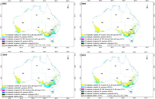
Figure 10. ACCA algorithm derived croplands (ACPs) for drought and non-drought years for Australia. Croplands versus cropland fallows computed using ACCA algorithm are shown for two: (a) worst drought years: 2002 and 2006 (ACP2000 and ACP2006), (b) normal years: 2003 and 2004 (ACP2003 and ACP2004), and (c) good years: 2000 and 2010 (ACP2000 and ACP2010).

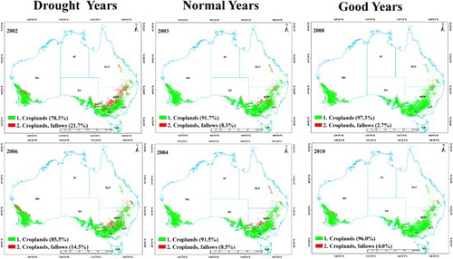
Figure 11. ACP2000 to ACP2015 derived cropland areas versus cropland fallow areas.

Note: the dotted lines indicate mean of 16 years.

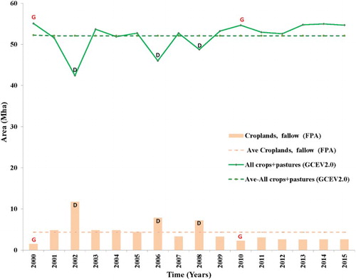
Figure 12. Cropland vigor during worst drought years versus the best above normal years. Mean MODIS 250 m NDVIs of Australia’s croplands during the: (a) three worst drought years of the century (2002, 2006, and 2008) versus (b) two very good years (2000 and 2010).

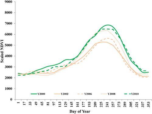
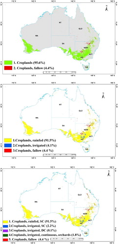
Figure 13. Cropland products of Australia. (a) Product 1: croplands versus non-croplands; (b) Product 2: irrigated versus rainfed; and (c) Product 3: cropping intensity: croplands with single, double, or triple cropping as well as cropland fallows.

Salmon, J. M., M. A. Friedl, S. Frolking, D. Wisser, and E. M. Douglas. 2015. “Global Rain-fed, Irrigated, and Paddy Croplands: A new High Resolution map Derived From Remote Sensing, Crop Inventories and Climate Data.” International Journal of Applied Earth Observation and Geoinformation 38: 321–334. doi: 10.1016/j.jag.2015.01.014

 Web of Science ®Google Scholar

Australian Bureau of Statistics. 2008. “ Water use on Australian Farms”, 2005-06 ca# 4618.0 http://www.abs.gov.au/AUSSTATS.

 Google Scholar