A general-purpose framework for parallel processing of large-scale LiDAR data

Figures & data

Figure 1. Architecture of the framework.

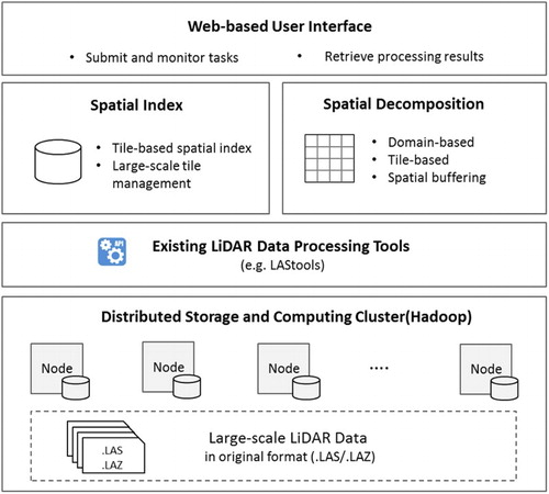
Figure 2. LiDAR data tiles for Colleton County, South Carolina.

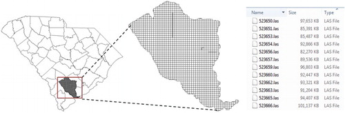
Figure 3. Structure of the tile-based spatial index linking a tile’s (T_i) file-space, geographic-space, and cluster-space.

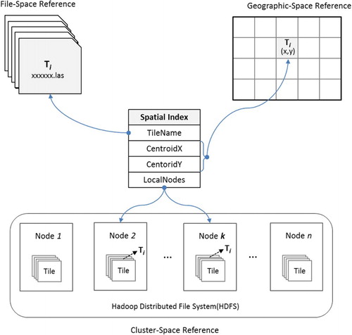
Figure 4. Illustration of domain-based spatial decomposition.

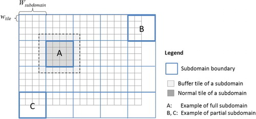
Figure 5. The distribution of the subdomain tiles in geographic-space and cluster-space with the two different decomposition mechanisms: (A) domain-based decomposition and (B) tile-based decomposition.

Note: The number in each tile (cell) indicates the computer node that tile is stored (i.e. 1 means the tile is stored on node1).

Figure 6. Integrating spatial decomposition with MapReduce and LAStools to implement tile-level parallelization.

Note: A Map in this figure refers to the map function of MapReduce.

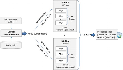
Figure 7. An example of the XML-based Job Description.

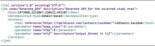
Figure 8. The online user interface of the prototype and the tile boundaries (red rectangles) of the LiDAR data for Colleton County in South Carolina.

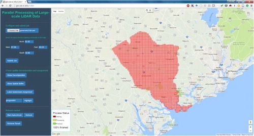
Figure 9. Job description file for the gridding operation.

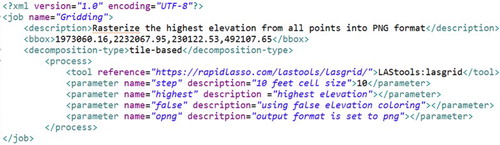
Figure 10. Snapshot of the job status: (A) generating DEM with domain-based decomposition (blue rectangles represent subdomains) and (B) rasterizing tiles with tile-based decomposition.

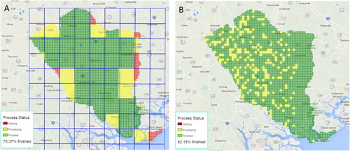
Figure 11. Subdomain assignment status for the two jobs with node7 highlighted: (A) generating DEM with domain-based decomposition and (B) rasterizing tiles with tile-based decomposition.

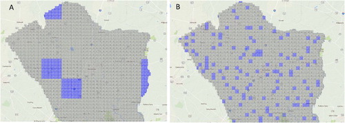
Figure 12. Manipulation of the results: (A) publishing the processed tiles as a data service; (B) mapping the data service to a computer Network Drive; (C) loading the processed tiles into ArcMap to conduct further process such as mosaic; and (D) displaying the processed tiles in Google Earth. (Note that the tiles displayed in ArcMap and Google Earth are not yet seamlessly mosaicked, so the color discontinuity exists between different tiles from different class intervals.)

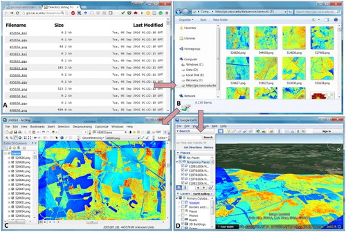
Table 1. Processing time (in second) for the two operations.

	Standalone	Cluster	Speedup
Gridding operation	2423	261	9.28
DEM operation	3891	723	5.38

Figure 13. Time spent on the two operations using both the standalone tool and the cluster system when gradually increasing the data volume from 200 to 1378 tiles.

Note: For the case of 1378 tiles, the previous results were used.

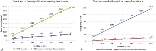
Figure 14. Speedup of using the prototype when gradually increasing the data volume for both operations.

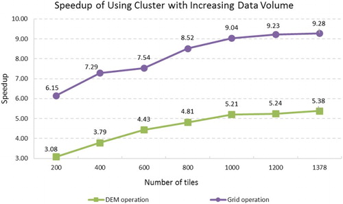
Figure 15. Time spent on gridding operation (A) and its corresponding speedup (B) with different number of nodes under different data volume scenarios.

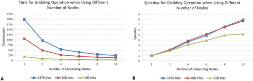
Figure 16. Number of points processed per second when conducting gridding operation for 1378 tiles.

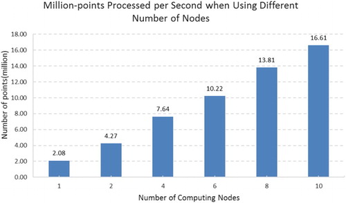
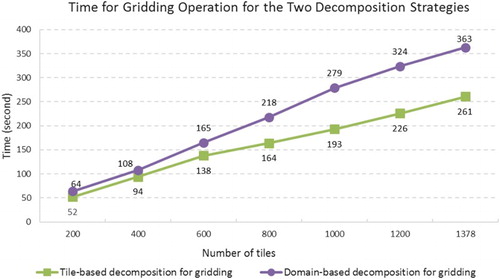
Figure 17. Comparison of tile-based decomposition and domain-based decomposition.