Figures & data
Figure 1. The main components of the geographic automata system and their interactivity in simulation (hollow boxes indicate data and data structures, filled boxes indicate models).
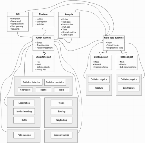
Figure 2. The path-planner can produce shortest paths between origins and destinations in the simulated space by imposing a graph of traversable area around buildings and building damage. Above, a circle indicates an HA-character’s position in the graph traversal pipeline, blue lines denote trip paths produced by the planning heuristic, the yellow grid denotes the global graph of traversable space, and black polygons denote building and debris envelopes.
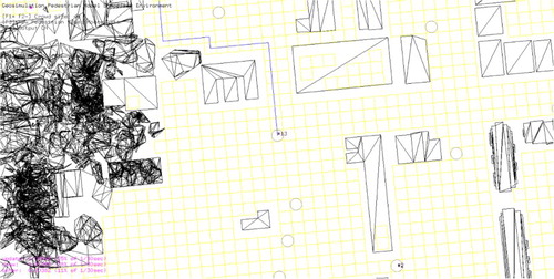
Figure 3. Left: the timeline for walker #307 in the LP scenario is illustrated, showing an extended period of speedy egress (accommodated by a path that proceeds through a SEH), followed by slowing-down at the assembly site. Right (callout): the steering paths for HA in a portion of the urban space for the LP scenario. In the callout, all HA paths through the space are shown in gray, and walker #307′s complete egress path is illustrated with a trail of blue dots (dark to light blue indicates progressive time spent in the scenario). Built structures are shown as light blue polygons, and resolved SEHs are illustrated in orange.
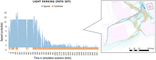
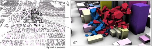
Figure 4. Left: A LiDAR-sourced volumetric model of Salt Lake City, UT was used to rapidly prototype a synthetic city environment for the simulation scenarios. We applied rolling tessellation and a rigid body physics engine to the volumetric model to produce collapse scenarios (right, inset in graphic above).
Table
Figure 5. Visualizations of space-speed paths for HA movement alongside walls shows HA-characters’ success in avoiding collisions with walls (as shown in the XY plane of movement), while also maintaining reasonable speed (visualized as the height (Z-plane) of the space-speed ribbons; higher ribbons indicates higher speed). Paths are color-coded by office cohort.
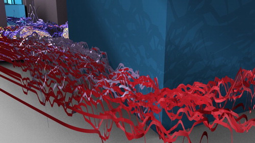
Figure 6. The influence of corners on egress: speed drops dramatically at the corner edge and a chain reaction of sorts forms in successive movement, locked-in at the corner. One can see a hole form in the collective space-speed path around the corner in a teardrop shape, with the collective heading forming the apex of the teardrop. (The yellow number 1 indexes the vantage point in to follow later in the paper.).
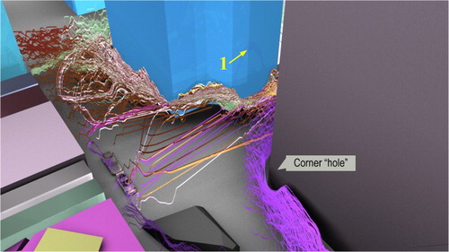
Figure 7. The influence of urban corridors, showing long-lived persistent movement through alleyways in locations of the urban scene that have linear corridors (top), but sloshing and slaloming effects in others where corridors are irregular (bottom). (The yellow number 2 indexes the vantage point in to follow later in the paper.).
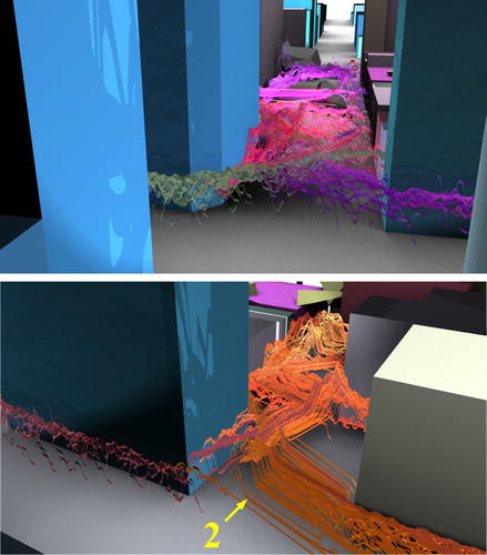
Figure 8. A system-wide view of shortest-paths from a few select origin locations in the simulated space (dots represent paths in the image above, color-coded by HA; gray polygons illustrate built infrastructure and damage debris). Local views are shown in the inset image, and HA perspectives on these views are shown in .
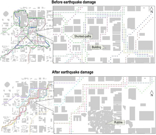
Figure 9. Space-speed paths around a large debris obstacle following building collapse, for the LP scenario. Walkers that initially steer to the left hand side of the obstacle establish a following phenomenon. (The yellow number 3 indexes the vantage point in to follow later in the paper.).
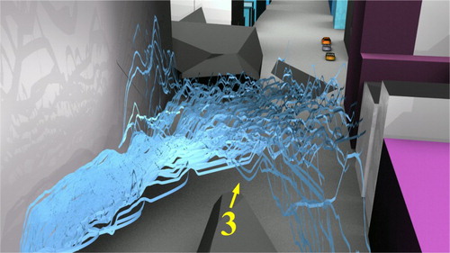
Figure 10. Individual shifts in behavior can catalyze broader phenomena. Above, a stream of successful collision avoidance alongside parked cars is interrupted suddenly when a HA walks, head-on, into the lane of like-moving HA that has formed. This creates an abrupt initial collision that must be resolved, which begets more and more collisions down-stream throughout the lane of moving pedestrians. Down-stream HA have little space to move and do not have information about the collision ahead of them. In slowing-down, successively through the phenomenon event-space, an initial log-jam turns into a larger congestion event, within a few seconds.
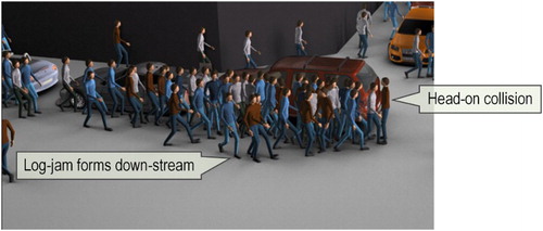
Figure 11. Walkers in the model must negotiate collisions with parked cars as they egress; the cars also block their vision, thereby limiting both their movement choices and the information that they can acquire around them. The top image shows space-speed paths of egress in the HP scenario: walkers avoid car-lined streets and their egress is funneled into the road. The bottom image presents a walker-based view of the surroundings, showing the visual blockage that parked cars create in egress.
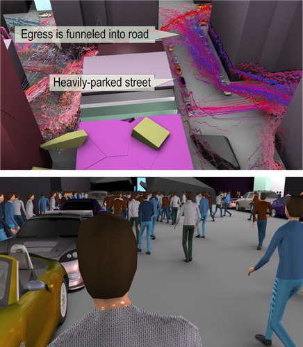
Table 1. Summary statistics for all SEHs, per alpha value (α), for the parking scenarios.
Table 2. Summary statistics for all walker paths for the parking scenarios.
Figure 12. The two parking scenarios (LP in the top image, HP in the bottom image) produce different SEHs. (The yellow numbers index vantage points from figures introduced earlier in the paper.).
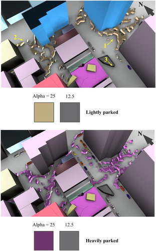
Figure 13. Left: the timeline for walker #263 in the HP scenario is illustrated, showing stop-and-go movement relative to persistent collisions over a small range of egress. Right (callout): the movement path for motile #263 is shown in blue (dark to light blue indicates progressive time spent in the scenario; gray lines indicate all HA movement paths; pink polygons represent resolved SEHs). (Compare this to the movement and timeline in .).
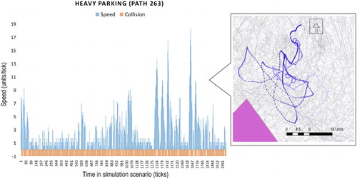
Table 3. Movement metrics for scenario-simulated paths.
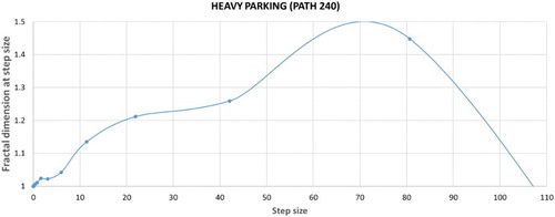
Figure 14. Fractal dimension variation at different step-size generalizations for walker #240 in the heavily-parked scenario, outside a SEH at an alpha value of 25. (The data points are not continuous; the connecting line is used solely for illustration because of the varying value range.).