Figures & data
Figure 1. Map of the study area and the distribution of the WSN nodes (projection: WGS_1984_UTM_Zone_47N)
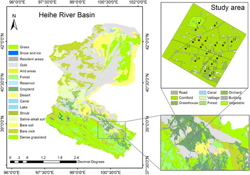
Figure 2. Time series of surface albedo over different surface types and the same surface type. (a) Time series of albedos from a cornfield, a building, an orchard, and a vegetable field. (b) Albedo values from different cornfields.
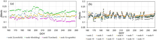
Table 1. List of coarse-scale albedo products used in this study.
Figure 3. Flowchart of the proposed method for establishing the spatiotemporal trend surface and the corresponding upscaling method.
Figure 4. The OLS regression model between the CASI albedo and ground-based albedo and the results of a significance test.
Figure 5. The OLS regression models’ coefficients between the WSN-based albedos for each two neighbouring clear days.
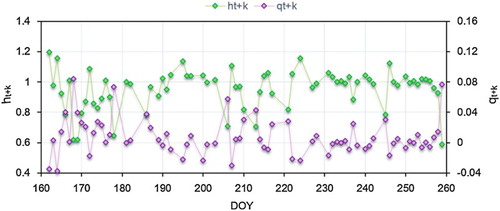
Figure 6. The R2 and significance test results of the OLS regression models between the WSN observed albedo on each two neighbouring clear days.
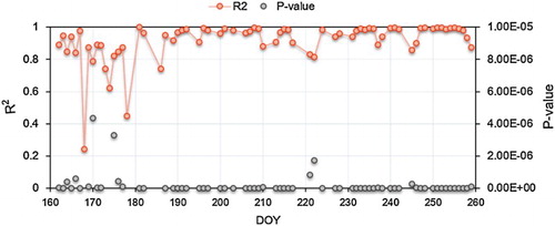
Figure 7. The spatial consistency between the trend surface and the ground-based measurements over the WSN nodes. Only the results for the initial and final days are shown for conciseness.
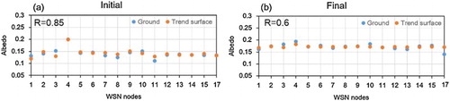
Figure 8. The temporal consistency between the trend surface and the ground-based measurements over different land cover types during the study period. Only one node within a cornfield is shown for conciseness.
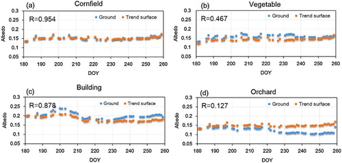
Figure 9. The trend surface (left) and the upscaling results with a 1-km grid (right) for the initial day (up) and the last clear day (down) during the study period.
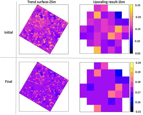
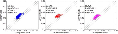
Figure 10. The scatterplots between the upscaling results and albedo products during the study period (from left to right, MODIS (V006), GLASS and MuSyQ).