Speckle filtering of Synthetic Aperture Radar images using filters with object-size-adapted windows

Figures & data

Figure 1. The samples contained in the smallest window have the standard deviation . As the window grows larger, the standard deviation decreases until it overlaps pixel(s) from the adjacent object(s).

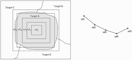
Figure 2. Flow chart of the proposed algorithm, filtering with adaptive window size.

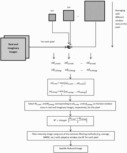
Figure 3. Near the edges of a target, the average filter with adaptive window size is not expected to work effectively. This is because as the filtering window overlaps parts of other targets before the window size becomes large enough to provide an accurate estimate of the backscattering coefficient.

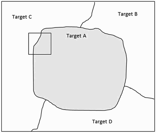
Figure 4. The selected subsets for applying the suggested filters: (A) San Francisco and (B) St. John’s.

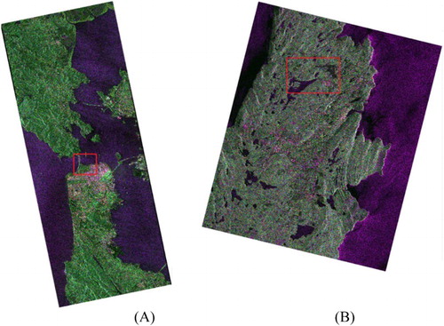
Figure 5. The block diagram of the simulation method.

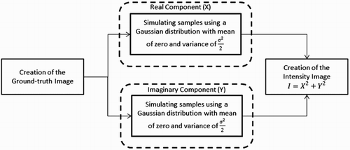
Figure 6. Simulated SAR images: (A) the ground-truth images, (B) the original intensity images, (C) the 5 × 5 average filtered images, (D) the 5 × 5 MMSE (Lee 1980, 1981a) filtered images, (E) average filtered images with adaptive window size, and (F) MMSE filtered images with adaptive window size.

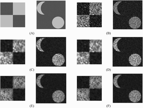
Table 1. Various indices for evaluation and comparison of the performance of the proposed speckle filters on the simulated SAR images.

	MSE		SNR		SSIM
	1st Image	2nd Image	1st Image	2nd Image	1st Image	2nd Image
Average filter	0.0537	0.0556	−1.2773	−3.3865	0.7086	0.6503
MMSE filter (Lee 1980, 1981a)	0.0565	0.0567	−1.5007	−3.4727	0.6905	0.6408
Average filter with adaptive window size	0.0815	0.0686	−3.0921	−4.2946	0.6519	0.6208
MMSE filter with adaptive window size	0.0813	0.0685	−3.0775	−4.2894	0.6429	0.6151

Figure 7. San Francisco: (A) original one-look HH intensity image. The rectangle on the top and the bottom of the image show the regions used for computation of ENL and coefficient of variation, respectively, (B) the 5 × 5 average filtered image, (C) the 5 × 5 MMSE (Lee 1980, 1981a) filtered image, (D) the 5 × 5 enhanced Lee (Lopes, Touzi, and Nezry 1990) filtered image, (E) the 5 × 5 Gamma (Lopes et al. 1993) filtered image, (F) PPB (Deledalle, Denis, and Tupin 2009) filtered image with hw = 20, hd = 5, and 1 iteration, (G) average filtered image with adaptive window size, and (H) MMSE filtered image with adaptive window size.

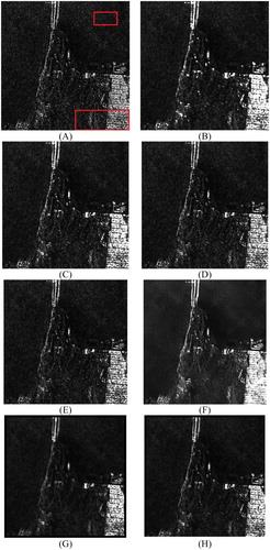
Figure 8. St. John’s: (A) original one-look HH intensity image. The rectangle on the top and the bottom of the image shows the regions used for computation of coefficient of variation and ENL, respectively, (B) the 5 × 5 average filtered image, (C) the 5 × 5 MMSE (Lee 1980, 1981a) filtered image, (D) the 5 × 5 enhanced Lee (Lopes, Touzi, and Nezry 1990) filtered image, (E) the 5 × 5 Gamma (Lopes et al. 1993) filtered image, (F) PPB (Deledalle, Denis, and Tupin 2009) filtered image with hw = 10, hd = 3, and 4 iterations, (G)average filtered image with adaptive window size, and (H) MMSE filtered image with adaptive window size.

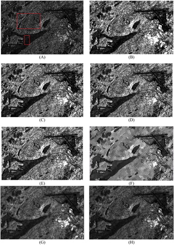
Figure 9. The variation in standard deviation with the change in the filtering window size. (A) A homogeneous pixel and (B) a heterogeneous pixel.

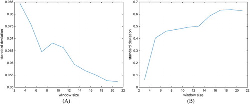
Table 2. Various indices for evaluation and comparison of the performance of the proposed speckle filters on real SAR images.

Image	San Francisco				St. John’s
	ENL				ENL
Original image	0.9233	2.6284	1	1	0.8919	0.8908	1	1
Average filter	11.2384	1.7112	0.9663	0.9564	10.4493	0.7713	0.9653	0.9563
MMSE filter (Lee 1980, 1981a)	7.2548	2.8251	0.9100	0.7612	7.0836	0.9611	0.9086	0.7637
Enhanced Lee filter (Lopes, Touzi, and Nezry 1990)	6.0499	3.7046	0.9360	0.7528	5.7243	1.0963	0.9317	0.7572
Gamma filter (Lopes et al. 1993)	6.8299	4.0011	1.0051	0.8108	5.7897	1.1009	1.0062	0.8079
PPB filter (Deledalle, Denis, and Tupin 2009)	6.9235	2.4647	0.6149	0.5231	5.7930	0.7014	0.7760	1.5383
Average filter with adaptive window size	10.4822	1.003	1.1394	1.5280	10.2089	0.7065	1.1356	1.4085
MMSE filter with adaptive window size	9.3041	2.7543	1.0037	0.9078	9.3788	0.8479	1.0152	0.8793

Figure 10. San Francisco: ratio images resulted from: (A) the 5 × 5 average filtered image, (B) the 5 × 5 MMSE (Lee 1980, 1981a) filtered image, (C) the 5 × 5 enhanced Lee (Lopes, Touzi, and Nezry 1990) filtered image, (D) the 5 × 5 Gamma (Lopes et al. 1993) filtered image, (E) PPB (Deledalle, Denis, and Tupin 2009) filtered image with hw = 20, hd = 5, and 1 iteration, (F) average filtered image with adaptive window size, and (G) MMSE filtered image with adaptive window size from the San Francisco image.

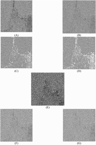
Figure 11. St. John’s: ratio images resulted from: (A) the 5 × 5 average filtered image, (B) the 5 × 5 MMSE (Lee 1980, 1981a) filtered image, (C) the 5 × 5 enhanced Lee (Lopes, Touzi, and Nezry 1990) filtered image, (D) the 5 × 5 Gamma (Lopes et al. 1993) filtered image, (E) PPB (Deledalle, Denis, and Tupin 2009) filtered image with hw = 10, hd = 3, and 4 iterations, (F) average filtered image with adaptive window size, and (G) MMSE filtered image with adaptive window size from the San Francisco image.

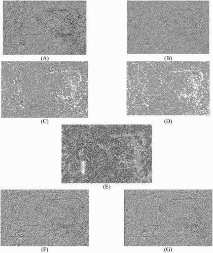
Figure 12. A small subset of the San Francisco image (A) original one-look HH intensity image, (B) the 5 × 5 average filtered image, (C) the 5 × 5 MMSE (Lee 1980, 1981a) filtered image, (D) the 5 × 5 enhanced Lee (Lopes, Touzi, and Nezry 1990) filtered image, (E) the 5 × 5 Gamma (Lopes et al. 1993) filtered image, (F) PPB (Deledalle, Denis, and Tupin 2009) filtered image with hw = 20, hd = 5, and 1 iteration, (G) average filtered image with adaptive window size, and (H) MMSE filtered image with adaptive window size highlighting urban areas from the San Francisco image.

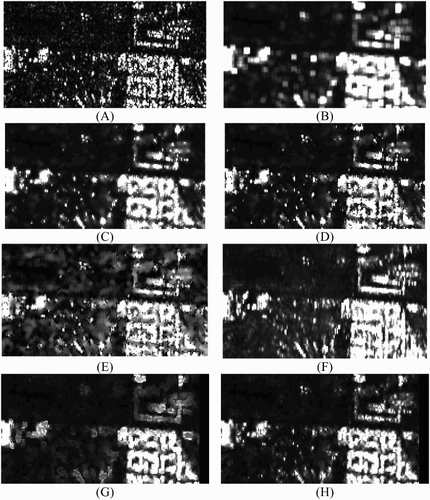
Figure 13. A small subset of St. John’s (A) original one-look HH intensity image, (B) the 5 × 5 average filtered image, (C) the 5 × 5 MMSE (Lee 1980, 1981a) filtered image, (D) the 5 × 5 enhanced Lee (Lopes, Touzi, and Nezry 1990) filtered image, (E) the 5 × 5 Gamma (Lopes et al. 1993) filtered image, (F) PPB (Deledalle, Denis, and Tupin 2009) filtered image with hw = 10, hd = 3, and 4 iterations, (G) average filtered image with adaptive window size, and (H) MMSE filtered image with adaptive window size highlighting urban areas from the St. John’s image.

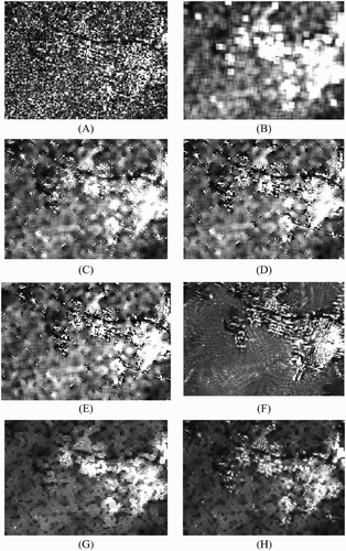
Figure 14. Simulated PolSAR images: (A) the ground-truth images, (B) the original polarimetric images, (C) the 5 × 5 average filtered images, (D) Images filtered with 5 × 5 refined PolSAR filter (Lee, Grunes, and De Grandi 1999), (E) average filtered images with adaptive window size, and (F) PolSAR filtered images with adaptive window size.

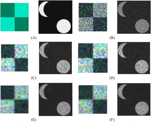
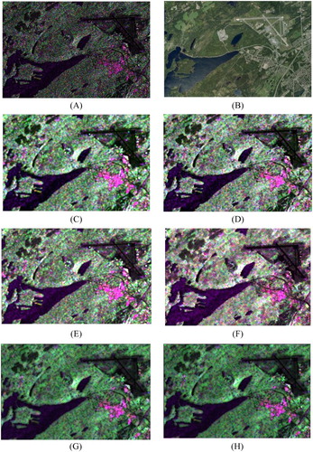
Figure 15. San Francisco: (A) original polarimetric image, (B) snapshot of the study area from Google Earth^TM, (C) the 5 × 5 average filtered image, (D) image filtered with 5 × 5 refined PolSAR filter (Lee, Grunes, and De Grandi 1999), (E) the 5 × 5 Lopez (Lopez-Martinez and Fabregas 2008) filtered image, (F) IDAN (Vasile et al. 2006) filtered image with window size row of 50, (G) average filtering with adaptive window size, and (H) PolSAR filtering with adaptive window size.

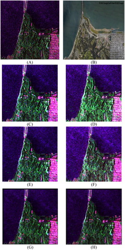
Figure 16. St. John’s: (A) original polarimetric image, (B) snapshot of the study area from Google Earth^TM, (C) the 5 × 5 average filtered image, (D) image filtered with 5 × 5 refined PolSAR filter (Lee, Grunes, and De Grandi 1999), (E) the 5 × 5 Lopez (Lopez-Martinez and Fabregas 2008) filtered image, (F) IDAN (Vasile et al. 2006) filtered image with window size row of 50, (G) average filtering with adaptive window size, and (H) PolSAR filtering with adaptive window size.

Lee, Jong-Sen. 1980. “Digital Image Enhancement and Noise Filtering by use of Local Statistics.” IEEE Transactions on Pattern Analysis and Machine Intelligence 2: 165–168. doi: 10.1109/TPAMI.1980.4766994

 PubMed Web of Science ®Google Scholar

Lee, Jong-Sen. 1981a. “Refined Filtering of Image Noise Using Local Statistics.” Computer Graphics and Image Processing 15 (4): 380–389. doi: 10.1016/S0146-664X(81)80018-4

 Google Scholar

Lopes, Armand, Ridha Touzi, and E. Nezry. 1990. “Adaptive Speckle Filters and Scene Heterogeneity.” IEEE Transactions on Geoscience and Remote Sensing 28 (6): 992–1000. doi: 10.1109/36.62623

 Web of Science ®Google Scholar

Lopes, A., E. Nezry, R. Touzi, and H. Laur. 1993. “Structure Detection and Statistical Adaptive Speckle Filtering in SAR Images.” International Journal of Remote Sensing 14 (9): 1735–1758. doi: 10.1080/01431169308953999

 Web of Science ®Google Scholar

Deledalle, Charles-Alban, Loïc Denis, and Florence Tupin. 2009. “Iterative Weighted Maximum Likelihood Denoising with Probabilistic Patch-based Weights.” IEEE Transactions on Image Processing 18 (12): 2661–2672. doi: 10.1109/TIP.2009.2029593

 PubMed Web of Science ®Google Scholar

Lee, Jong-Sen, Mitchell R. Grunes, and Gianfranco De Grandi. 1999. “Polarimetric SAR Speckle Filtering and its Implication for Classification.” IEEE Transactions on Geoscience and Remote Sensing 37 (5): 2363–2373. doi: 10.1109/36.789635

 Web of Science ®Google Scholar

Lopez-Martinez, Carlos, and Xavier Fabregas. 2008. “Model-based Polarimetric SAR Speckle Filter.” IEEE Transactions on Geoscience and Remote Sensing 46 (11): 3894–3907. doi: 10.1109/TGRS.2008.2002029

 Web of Science ®Google Scholar

Vasile, Gabriel, Emmanuel Trouvé, J. Lee, and Vasile Buzuloiu. 2006. “Intensity-driven Adaptive-Neighborhood Technique for Polarimetric and Interferometric SAR Parameters Estimation.” IEEE Transactions on Geoscience and Remote Sensing 44 (6): 1609–1621. doi: 10.1109/TGRS.2005.864142

 Web of Science ®Google Scholar