Figures & data
Figure 1. Three types of artificially generated patterns for a fixed partition of ‘settlement’ and ‘non-settlement’ pixels: the pattern represented by (a) is a perfectly compact pattern consisting of one single, contiguous patch, (b) shows two examples for fragmented and clustered patterns, both consisting of many patches with different sizes and (c) is a perfectly dispersed pattern without coalescent patches forming not even one larger patch; as a consequence, any pixel has the same size.
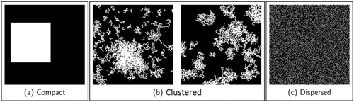
Figure 2. Schematic illustration of the model design for ranking binary patterns with respect to their spatial dispersion. Each arbitrary binary and two-dimensional pattern can be unambiguously located within the feature space of the model, which is defined only by two parameters, the NP on the x-axis and the LP on the y-axis.
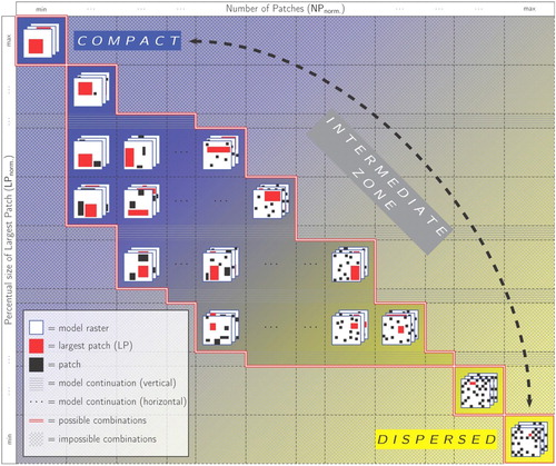
Figure 3. Examples for artificial patterns and the corresponding values for the NP, NPn, LP, LPn and DI. White pixels = class ‘1’, red Pixels (in print darker pixels) = largest patch of class ‘1’, and black pixels = background. NP = absolute number of patches; LP = percent area of the largest patch; NPn = normalized number of patches (relative); LPn = normalized percent area of the largest patch (relative).
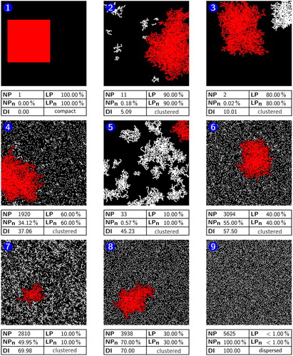
Figure 4. Two-dimensional feature space spanned by the parameters NPn and LPn. The numbered points symbolize the locations within the model of the related patterns displayed in . The ‘area of impossible parameter combinations’ is because the value of the NPn determines the corresponding parameter LPn and vice versa.
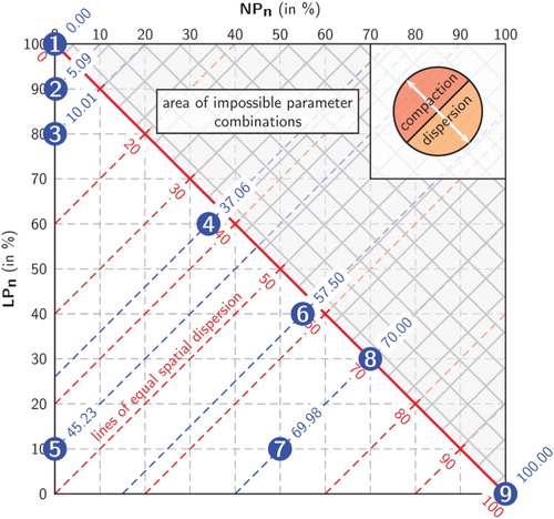
Figure 5. Behavior of the Landscape Shape Index (LSI) for (a) an increasing grade of dispersion caused by rising NPn and constant LPn of 20% and (b) for a decreasing grade of dispersion caused by rising LPn and constant NPn of 8.87% (500 patches).
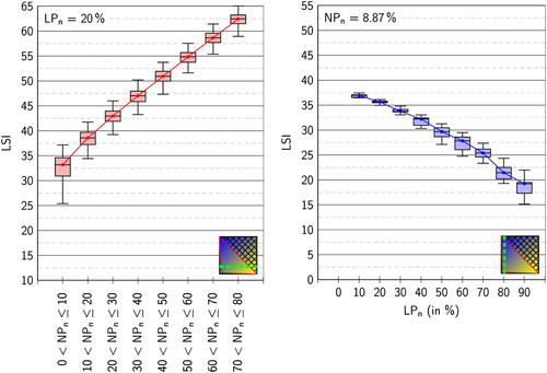
Table 1. 26 selected class-level metrics and their behavior regarding monotony in horizontal respectively vertical direction within the model.
Figure 6. Influence of the spatial extent and spatial resolutions onto the dispersion index.
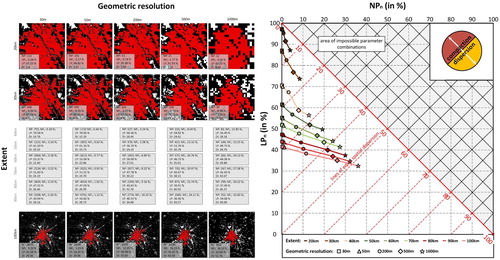
Figure 7. Binary settlement patterns for the cities Shenzhen and Dongguan in China, Frankfurt am Main and Cologne in Germany and Warsaw in Poland at four different time steps (1975, 1990, 2000, 2010). Areas that are covered by settlement elements are displayed in white. The largest urban patch (LP) is visualized in grey. The dimension of each frame is 30 × 30 kilometers around a defined city center; the geometric resolution of each raster is 200 meters.
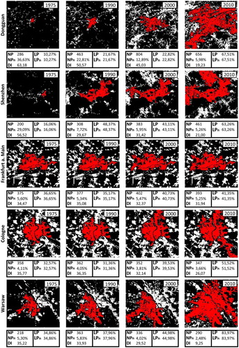
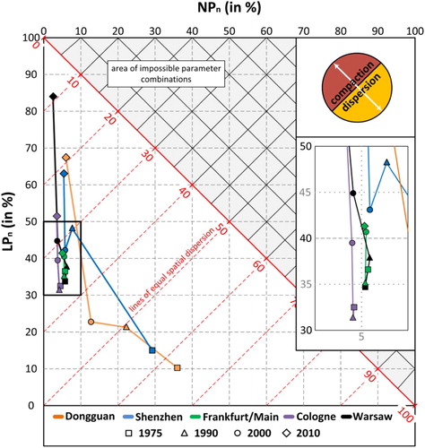
Figure 8. Shifts in dispersion for the five sample cities within the two-dimensional feature space spanned by the parameters NPn and LPn.