Figures & data
Figure 1. Schema of the construction of a kernel function K between regions and
.
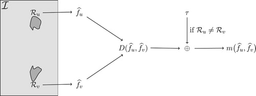
Figure 2. The experiment design overview.
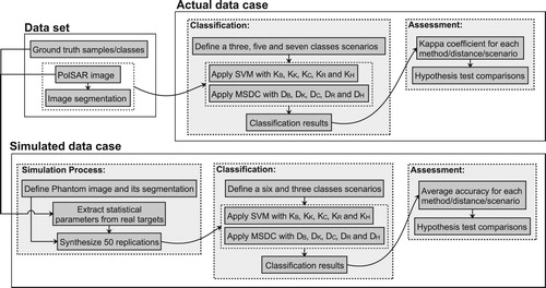
Figure 3. The study area, actual PolSAR image and the spatial distribution of the LULC samples used in the study. (a) Study area location, (b) ALOS-PALSAR image in RGB color composition (HH, HV, VV) and (c) LULC samples.
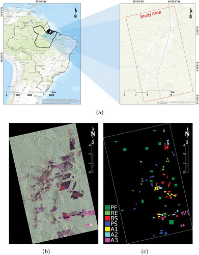
Figure 4. Simulated data. (a) Phantom - Blocks, (b) Simulation example and (c) Mean covariance matrices (squares), and 44 perturbed covariance matrices (circles) in semilogarithmic scale.
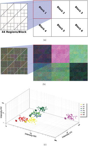
Figure 5. Simulated data. (a) Training samples – six classes case, (b) Ideal result for six classes, (c) Training samples – three classes case and (d) Ideal result for three classes.

Figure 6. The accuracy of classification results for the simulated data set. (a) Six classes classification and (b) Three classes classification.
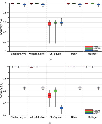
Table 1. Test statistic p-values for the t test that verifies that two classification techniques produce equivalent results. Values above (below) the diagonal correspond to the six (three, resp.) classes. Underlined values indicate equivalent coefficients at the 95% level.
Figure 7. The computational of the analyzed methods in the expriment with synthetic data.
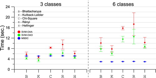
Table 2. Summary of the land cover classes samples.
Figure 8. Spatial distribution of the samples on the different considered scenarios and the adopted segmentation. (a) Scenario 1, (b) Scenario 2, (c) Scenario 3 and (d) Segmentation.
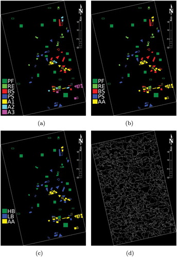
Figure 9. Classification accuracy.
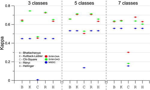
Table 3. p-values from hypothesis test for comparing methods and distances with seven classes. Underlined values indicate equivalent coefficients at the 95% level.
Table 4. p-values from hypothesis for comparing methods and distances with five classes. Underlined values indicate equivalent coefficients at the 95% level.
Table 5. p-values from hypothesis tests for comparing methods and distances with three classes. Underlined values indicate equivalent coefficients at the 95% level.
Figure 10. Actual data classification results. (a) SA/B – Scenario 1, (b) SO/K – Scenario 1, (c) MS/R – Scenario 1, (d) SA/H – Scenario 2, (e) SO/R – Scenario 2, (f) MS/K – Scenario 2, (g) SA/R – Scenario 3, (h) SO/K – Scenario 3 and (i) MS/H – Scenario 3.
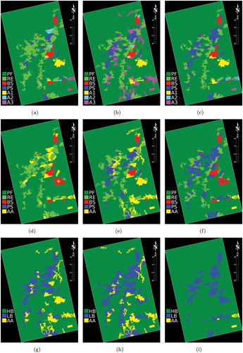
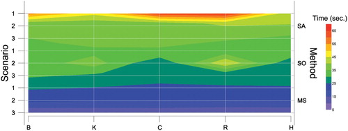
Figure 11. Computational time of the analyzed methods in the experiment with actual data.