Figures & data
Figure 1. GSM cells in the Brno city area. The spatial resolution of cells is highly variable, the most detailed being in the city centre (GSMWEB Citation2018).
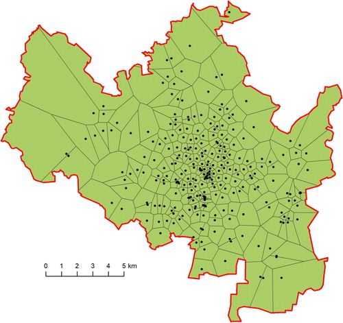
Table 1. Differences of the population between census data and current estimated population. The numbers for 2020 were estimated in a demographic analysis. Adapted from Seidenglanz, Toušek, and Chvátal (Citation2013, 26).
Figure 2. Localization of the pilot area (yellow) within the Brno. Selected spatial units: 1 – Náměstí Svobody’, 2 – ‘Janáčkovo divadlo’, 3 – ‘Zelný trh’, and 4 – ‘Přízová’.
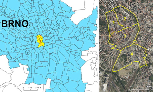
Figure 3. Temporal variability of estimated human presence (spatial unit no. 1 – ‘Náměstí Svobody’).
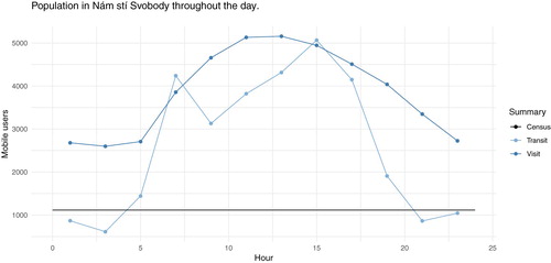
Figure 4. Functional delimitation of buildings in Brno centre (a – building type; and b – number of floors).
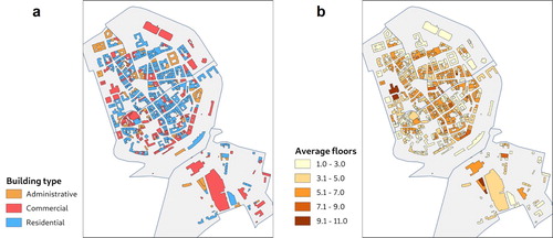
Table 2. Weights per functional delimitation and day/night.
Figure 5. Details of analytical maps (a – PR+PNR; b – PR+PNR; and c – PR+PNR+PT).
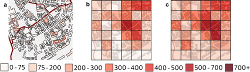
Figure 6. Schematic description of the procedure used for building level dasymetric population.
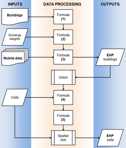
Figure 7. Census population compared to night and day averages of BEHP population (mobile phone data, PR+PNR) in individual buildings. Buildings are ordered by the value of BEHP population. Building order n denotes n-th building with the largest population in a given series.
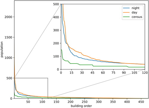
Figure 8. Frequency distribution of buildings from census data compared to day and night averages of BEHP population (mobile phone data). Axis X = category of buildings by population.
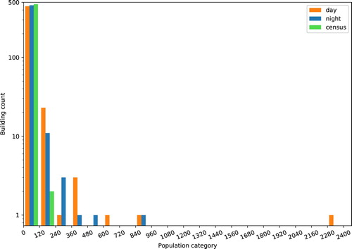
Figure 9. Analytical maps for three methods (a – PR+PNR on building level; b – PR+PNR on grid level; and c – PR+PNR+PT on grid level) and selected hours.
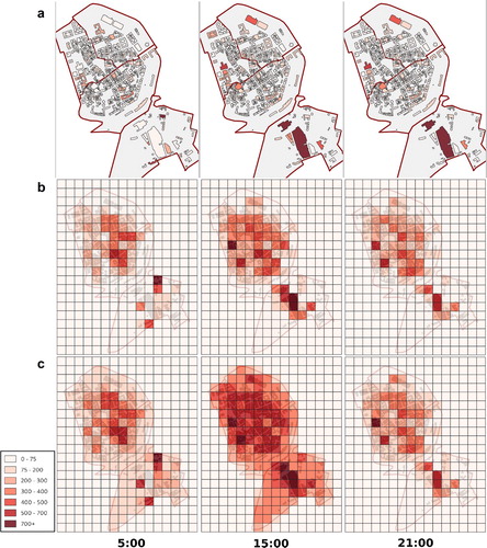
Figure 10. The difference for residential buildings between building level average BEHP (PR+PNR) and census data for day (a) and night (b).
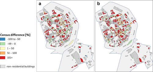
Figure 11. Building level BEHP (PR+PNR) average for day (a) and night (b).
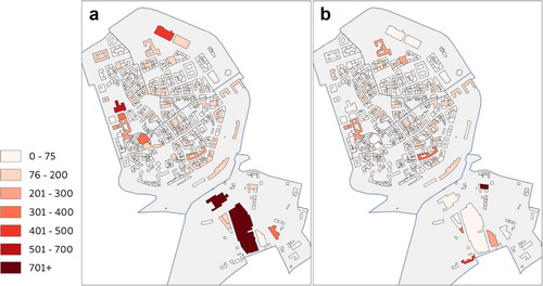
Figure 12. Average number of PR+PNR+PT for day (a) and night (b) for a grid data.
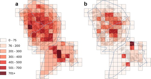
Figure 13. Average number of visitors (PR+PNR) for day (a) and night (b) for a grid data.
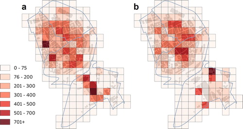
Figure 14. Comparison of PR (residents) and PN+PNR (visitors) data for day (a) and night (b) for a grid data.
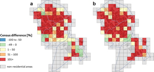
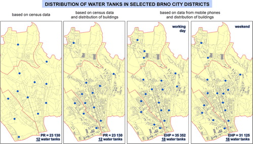
Figure 15. The role of spatio-temporal distribution of population in the case of water shortage (see the text for a detailed description).