Figures & data
Figure 1. Simulated 3D view of a real passenger aircraft (GS7581) flying over Tianjin, China from Flightradar24 (Flightradar24 Citation2020).
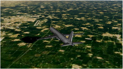
Figure 2. (a) Global flying aircrafts distribution at 20:00 on 2019-12-06. Blue pins denote the airport locations. (b) Number of flights tracked per day from December 1 to December 14, 2019. Data are from (Flightradar24 Citation2020).
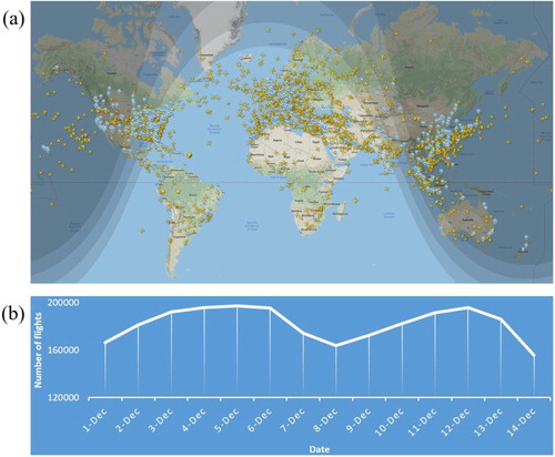
Figure 3. (a) Number of smartphone users from 2016 to 2019 (Data from Statista [Citation2020]). (b) Smartphone camera rank from 2013 to 2019 (Data from DXOMARK [Citation2020b]).
![Figure 3. (a) Number of smartphone users from 2016 to 2019 (Data from Statista [Citation2020]). (b) Smartphone camera rank from 2013 to 2019 (Data from DXOMARK [Citation2020b]).](/cms/asset/3a628644-05de-4993-a59d-fa681d08c4f8/tjde_a_1808721_f0003_oc.jpg)
Figure 4. Three typical accessories that can be used to facilitate image capturing (a) Flexible 360 clip mobile phone holder. (b) Sefie stick. (c) Gimbal Stabilizer.
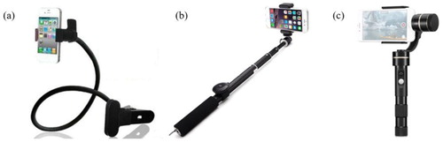
Figure 5. VPARS imaging geometry.
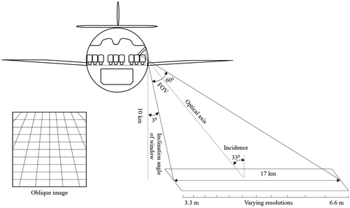
Figure 6. (a) Diagram of 1-D piecewise linear interpolation along time. (b) Piecewise linear interpolation of the discrete aircraft positions downloaded from FlightAware. Red points are the original flight tracking points with position information, and blue line is the flight trace interpolated from original flight tracking points.
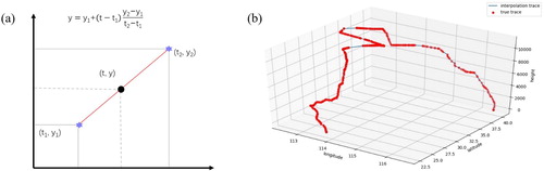
Figure 7. (a) Original hazy VPARS image, (b) dark channel of this image, and (c) restored haze-free VPARS image.
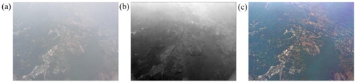
Figure 8. (a) VPARS image with cloud, (b) binary map of cloud masks, and (c) VPARS image with cloud masks.
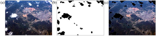
Figure 9. The flight information for the experiment. (a) Flight map. (b) Altitude and speed information of the flights.
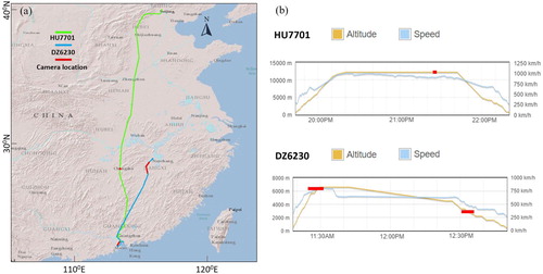
Table 1. The data collection details for the experiment.
Figure 10. Example of selecting GCPs in the image. These GCPS should better be: (1) located at corners of roads or land parcels; (2) distributed uniformly on the image; (3) on the ground.
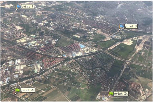
Figure 11. Results of daytime image processing. (a) Orthomosaic image of case 1. (b) Orthomosaic image of case 2.
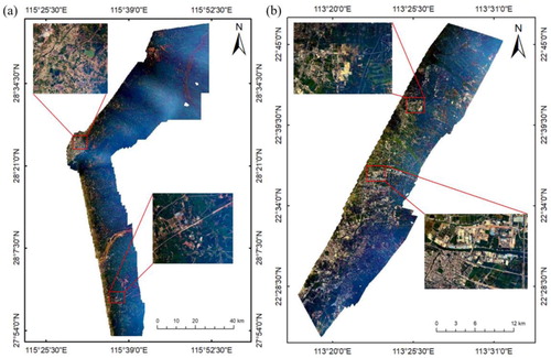
Figure 12. Clouds removed by taking advantage of images from multiple viewing angles. (a) Cartoon diagram showing how multiple-images are generated. (b) A case of removing cloud using images from multiple viewing angles. The rectangle indicates the cloudy area.
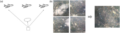
Table 2. Geometric accuracy of orthorectified images.
Figure 13. Samples of point clouds. (a) Rendered by true color. (b) Rendered by height.
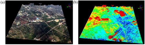
Figure 14. DEM results of case 1. (a) Histograms of elevation errors. (b) Height profile comparison. (c) Derived DEM from VPARS. (d) ASTER DEM for comparison.
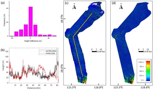
Figure 15. DEM results of case 2. (a) Histograms of elevation errors. (b) Height profile comparison. (c) Derived DEM from VPARS. (d) ASTER DEM for comparison.
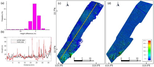
Figure 16. (a) Nighttime Imagery from VPARS. (b) The VIIRS Nighttime Imagery (Day/Night Band, Enhanced Near Constant Contrast) on July 1, 2018 downloaded from Worldview (NASA Citation2020a).
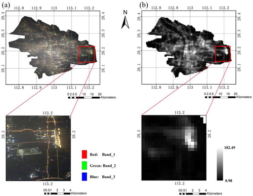
Figure 17. (a) Google Earth image. (b) VPARS orthomosaic image. (c) Classification based on a Google Earth image. (d) Classification based on VPARS orthomosaic image.
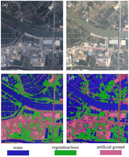
Figure 18. (a) POI density map in Changsha. (b) VPARS nightlight brightness map in Changsha. (c) POI grids with >10 POIs. (d) The regression analysis between nightlight brightness and POI number.
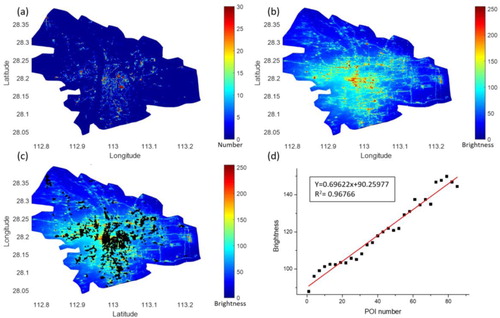
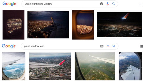
Figure 19. Several Google searching results using the keywords of ‘urban night plane window’ and ‘plane window land.’