Figures & data
Figure 1. Multilevel focus+context visualization of a DE.
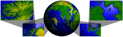
Figure 2. An initial polyhedron (a), is refined (b), and then projected to the sphere (c).
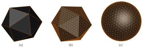
Figure 3. Overview of client and server responsibilities.
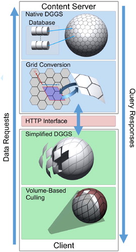
Figure 4. As opposed to a series of cell-based queries, a single tile-based query can request for all descendant cells at a desired resolution, reducing the cost of requesting those cells over the network.
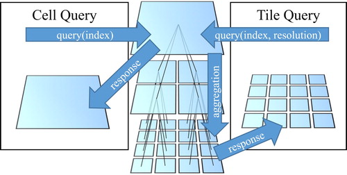
Figure 5. A particular tile's geometry sampled at different levels of detail – here the cusp on the left edge of the tile is caused by the subdivision method applied to the dual hexagonal grid on the server DGGS.
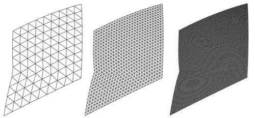
Figure 6. An example client–server cell refinement process.
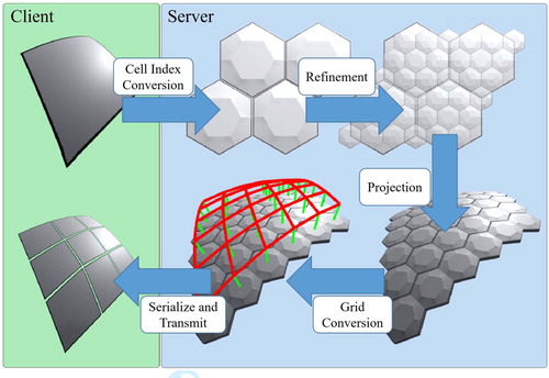
Table 1. Comparison between the number of tiles checked for visibility, tiles visible to a camera, the total number of DGGS tiles at various resolutions, and average time taken to download the tiles checked for visibility. Server and client DGGS prototypes were equipped with 3.2 GHz Intel® Core™ i7-8700 and 2.6 GHz Intel® Core™ i7-6700 CPUs, respectively, and 16 GB of RAM each.
Figure 7. Data textures shared between different visualizations (data sources: 1, 2, 4).
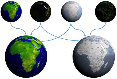
Figure 8. Topographical visualization with landmarks included as a normal perturbation to give location context (data sources: 1, 4).
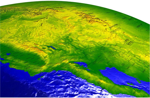
Figure 9. Various client-side data styling scenarios. (a) Artistic texture and styling emphasizing topography and bathymetry (data sources: 1, 3). (b) Map textures and embossed political boundaries (data sources: 1, 2, 4). (c) Population data and political boundaries as light-emitting textures (data sources: 1, 2, 5).
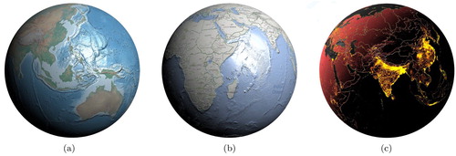
Figure 10. Three different visualizations of the same data but using different styling matrices (data sources: 1, 2, 3, 4, 5).
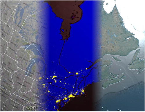
Figure 11. Canadian road networks in Alberta and Nova Scotia (data sources: 1, 8, 9). (a) These two road networks in Alberta and Nova Scotia cannot be viewed at high detail simultaneously without special techniques due to their distance and difference in scale. (b) Effective comparison of the road networks in Alberta and Nova Scotia utilizing multilevel focus+context visualization.
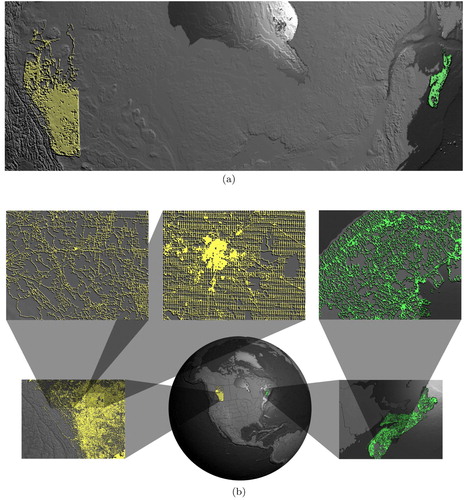
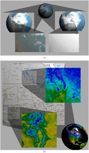
Figure 12. Multilevel focus+context visualization on the globe. (a) Population densities in different parts of the world (data sources: 1, 2, 5). (b) Calgary water bodies and flood projection (data sources: 4, 10, 11).
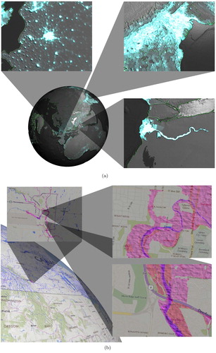
Figure 13. Multilevel focus+context visualizations which influence dataset styling. (a) Visualization comparing freezing point in winter versus spring (data sources: 1, 3, 6). (b) Mean temperatures for 2015, using a map dataset for context (data sources: 1, 4, 6).