Figures & data
Figure 1. Study area: Urban and peri-urban environment in Toulouse and its surroundings with a 2016 snapshot of the LULC.
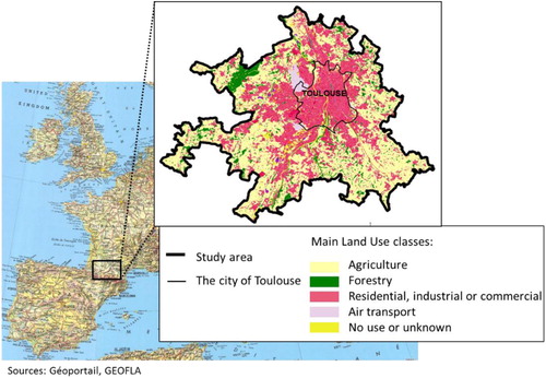
Figure 2. The spatial distribution of multi-source VGI collected in the study area
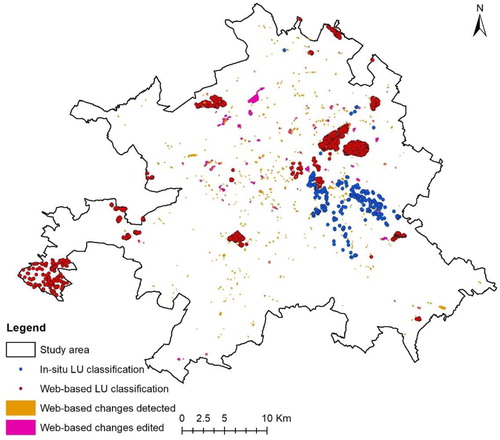
Figure 3. Classification of change detection observations: dominant label from contributors for web-based changes detected (blue bins) and web-based changes edited (red bins)
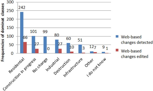
Figure 4. Distribution of LU classification chosen by contributors during the online mapping campaign
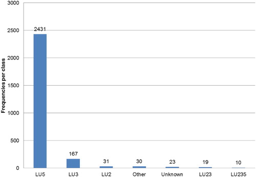
Table 1. A synthesis of data used in the present study.
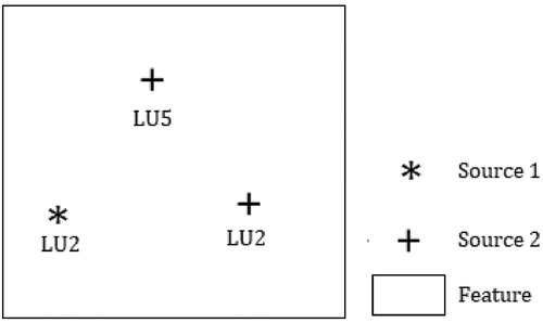
Figure 5. Illustration of six LU features characterized by (a) zero, (b) (c) one, (d) (e) two or (f) more observations coming from two data sources: Source 1 and Source 2. LU2 and LU5 refer to industrial use and residential use, respectively.
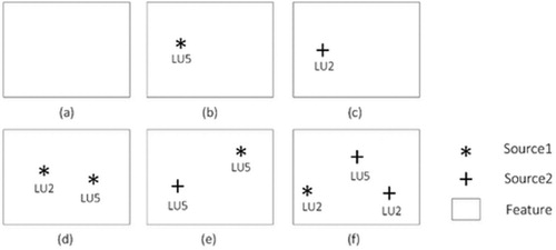
Figure 6. The workflow for updating authoritative LU data based on a multiple-source information fusion approach.
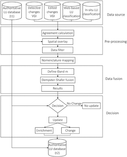
Figure 7. Example of managing overlaps between LU polygons and polygons derived from the change detection (CD) algorithm.
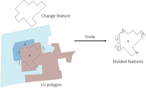
Figure 8. Examples of data filtering. (a) Geometry filtering (e.g. small divided CD polygons that overlap a road and contain potentially misleading change information); (b) Agreement filtering (e.g. CD polygon with an agreement value equal to 0); (c) Label-based filtering (e.g. a CD polygon with the label equal to ‘No change’)
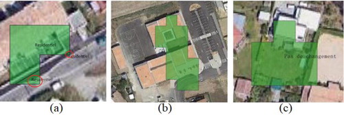
Table 2. Mapping labels of change features into the OCS-GE LU nomenclature.
Table 3. Mapping between the combined hypothesis and the singleton hypothesis.
Figure 9. The distribution of the number of contributions of the LU features collected. The number of LU features decreases as the number of observations increases (respectively, n=4081, 124, 19, 3 and 2). 96% have one contribution and 4% have between 2 and 5 contributions.
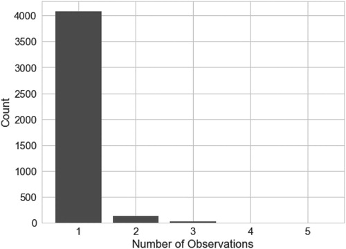
Figure 10. The overall accuracy and the number of LU polygons considered by confidence threshold values for features having two or more contributions.
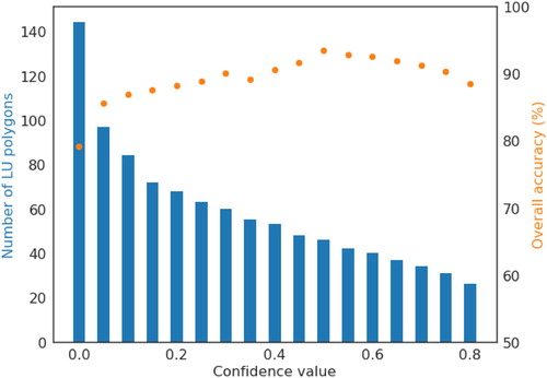
Table 4. Confusion matrix for features having two or more contributions with a confidence threshold greater than 0.05.
Figure 11. The LU polygons updated with the corresponding new LU labels. (LU2-Industrial, LU3-Commercial; LU4.1.1-Road transport; LU4.1.4-Water transport; LU5-Residential; LU6.1-Construction zones; LU6.3-Not currently used)
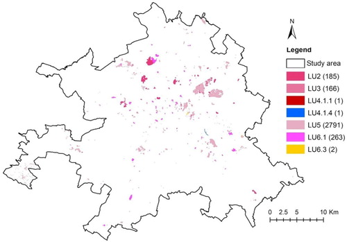
Figure 12. Examples of multi-source VGI collected for LU polygons. (a1-c1) LU polygons and associated multi-source VGI; (a2-c2) aerial imagery in 2016; (a3-c3) Pléiades imagery in 2019.
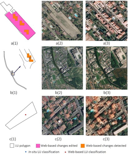
Figure 13. Examples of errors in the LU polygons from the multi-source VGI collected. The figures labelled (a) indicate a misclassification of new LU by the volunteers and those labelled (b) refer to a change that only covers part of the initial polygon. (a1-b1) LU polygons and associated data; (a2-b2) aerial imagery in 2016; (a3-b3) Pléiades imagery in 2019.
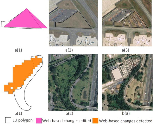
Table A1. Land cover nomenclature.
Table A2. Land use nomenclature.
Figure B1. An example of applying the proposed Dempster-Shafer fusion on a LU feature with three contributions from two sources