Figures & data
Figure 1. Schematic illustration of canopy cover (Dyer et al. Citation2014). Canopy cover is the fraction of ground covered by the vertically projected crown envelope (gray area), which is considered solid.
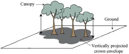
Figure 2. A sample of the effect of within-crown gaps on CC estimation. The CC was underestimated by approximately 50%, as many within-crown gaps were classified as non-canopy (i.e. gray pixels within the red outline). Note that reference canopy pixels were located in the canopy outlines that were manually delineated, and the reference CC was calculated as a ratio of the number of reference canopy pixels to the total pixels.
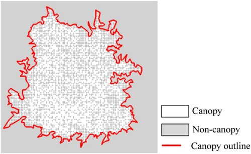
Figure 3. Location of the study area. Two of the UAV-LiDAR data acquisition sites (named as Plots 1 and 2) and corresponding forest types. Each of the two sites was divided into 12 samples, in which six samples containing roads are discarded (marked by black crosses).
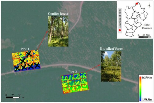
Figure 4. Distribution of canopy cover levels of Plots 1 and 2.
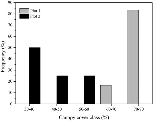
Table 1. Flight parameters and scanner properties of the UAV-LiDAR data acquisition.
Figure 5. Simulated point cloud data. (a) Canopy scene. (b) Samples of individual canopies with different proportions of within-crown gaps (10−60%).
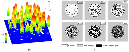
Figure 6. Overview of the cloth simulation method.
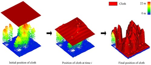
Figure 7. Canopy cover estimations with the (a) CHM and (b) pit-free CHM-based methods for all samples. The dashed line denotes a 1:1 relationship, and the solid line is the fitted line.
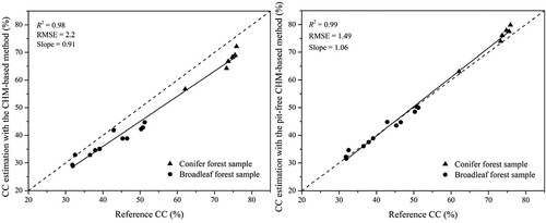
Table 2. Underestimation and overestimation errors of the CHM and pit-free CHM-based methods.
Figure 8. Error distributions of the (the first column) CHM and (the second column) pit-free CHM-based methods in Plots 1 and 2. (a) and (b) are Plot 1; (c) and (d) are Plot 2. In (a) and (b), blank rectangular regions are the discarded samples since they contain roads. In (c) and (d), regions inside the green circle represent the overestimation error caused by the inclined trunk.
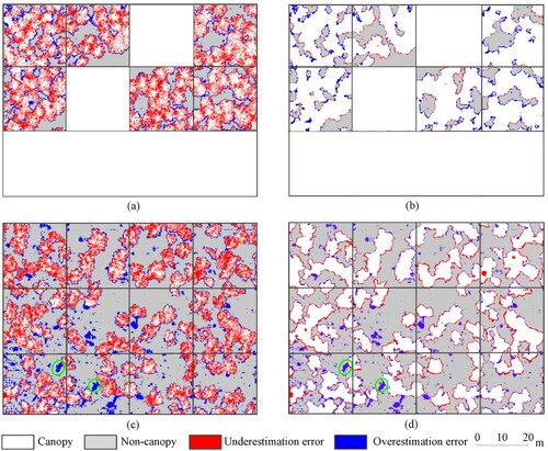
Figure 9. Influences of proportion of within-crown gaps (from 10% to 60%, with an interval of 10%) on the CC estimation accuracies for the CHM and pit-free CHM-based methods.
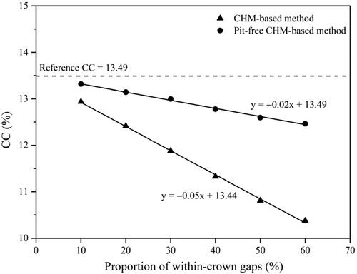
Figure 10. Error distribution of the CHM-based method at different proportions of within-crown gaps: (a) 10%, (b) 20%, (c) 30%, (d) 40%, (e) 50%, and (f) 60%. The region framed by the dashed rectangle is magnified on the underside.
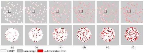
Figure 11. Error distribution of the pit-free CHM-based method at different proportions of within-crown gaps: (a) 10%, (b) 20%, (c) 30%, (d) 40%, (e) 50%, and (f) 60%. The region framed by the dashed rectangle is magnified on the underside.
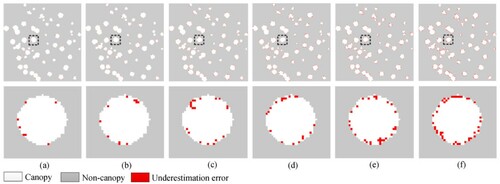
Figure 12. Canopy covers derived from different pixel sizes. (a) 0.07 m, (b) 0.13 m, (c) 0.21 m, and (d) 0.25 m.
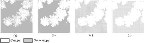
Figure 13. A sample with reference canopy sampling points overlaid on the CHM.
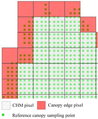
Figure 14. The sensitivity of the CHM-based method to the setting of pixel size.
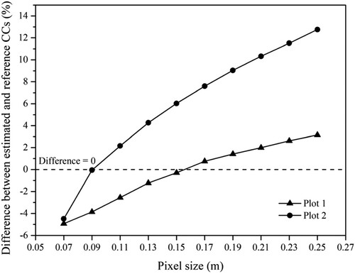
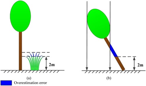
Figure 15. The distributions of overestimation error. (a) Understory vegetation. (b) Inclined trunk.