19-year remotely sensed data in the forecast of spectral models of the environment

Figures & data

Figure 1. Geographical location of Sinop – MT (A) and Passo Fundo – RS (B) and spatial variability of NDVI (product MOD13Q1.V6) of the temporal mean of the Julian days 206 to 258 of the year 2017, respectively.

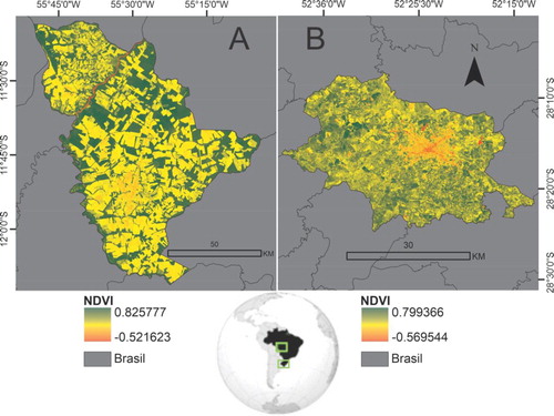
Table 1. Vegetation indices used in the study to estimate the soil management, in 2000/2001 and 2017/2018 crop years

Vegetation Index	Equations	References
Normalized Difference Vegetation (NDVI)	$NDVI={\displaystyle \frac{\rho NIR-\rho RED}{\rho NIR+\rho RED}}$	Rouse et al. (1974)
Enhanced Vegetation Index 2 (EVI2)	$EVI2=2.5\ast {\displaystyle \frac{\rho NIR-\rho RED}{\rho NIR+(2.4\ast \rho RED)+1}}$	Jiang et al. (2008)
Normalized Difference Senescence Index (NDSVI)	$NDSVI={\displaystyle \frac{\rho SWIR1-\rho RED}{\rho SWIR1+\rho RED}}$	Qi et al. (2002)
Soil Adjusted Total Vegetation Index (SATVI)	$SATVI={\displaystyle \frac{\rho SWIR1-\rho RED}{\rho SWIR1+\rho RED+L}(1+L)-\left({\displaystyle \frac{\rho SWIR2}{2}}\right)}$	Marsett et al. (2006)
Soil Tillage Index (STI)	$STI={\displaystyle \frac{\rho SWIR1}{\rho SWIR2}}$	Van Deventer et al. (1997)
Normalized Difference Tillage Index (NDTI)	$NDTI={\displaystyle \frac{\rho SWIR1-\rho SWIR2}{\rho SWIR1+\rho SWIR2}}$	Van Deventer et al. (1997)

Figure 2. Flowchart of the main steps of the study, with emphasis on GEOBIA and data mining in computing environments.

Table 2. Weight Coefficients ($\varpi$n) for the calculation of the planetary albedo through the use of LANDSAT-8 images.

Bands	Band 2	Band 3	Band 4	Band 5	Band 6	Band 7
$\varpi$n	0.300	0.277	0.233	0.143	0.036	0.012
ESUNλ,b	2011.3	1853	1532.8	956.4	237.8	80.2

Source: Silva et al. (2016) adapted by the authors.

Figure 3. Mapping of soybean (ha) in 2000/2001 (A and C) and 2017/2018 (B and D) crop years in the municipalities of Sinop -MT (A and B) and Passo Fundo-RS (C and D) by MODIS sensor.

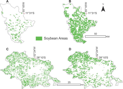
Figure 4. Vegetation indices for the 2017/2018 crop year in the municipalities of Passo Fundo-RS (A) and Sinop-MT (B).

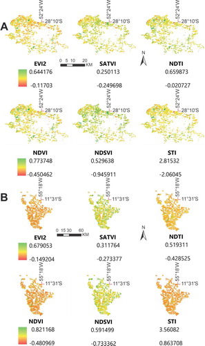
Figure 5. Segmentation and application of the decision tree in the municipalities of Passo Fundo-RS (A1/B1) and Sinop-MT (A2/B2) in the 2000/2001 and 2017/2018 crop years.

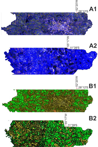
Figure 6. Discrimination of the areas studied regarding the type of soil management in 2000/2001 and 2017/2018 crop years. A – Passo Fundo and B – Sinop-MT.

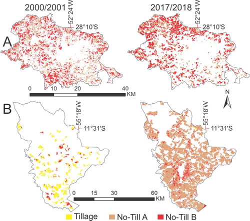
Table 3. Total area (ha) using tillage (T), no-till A (NT_A), and no-till B (NT_B) in the 2000/2001 and 2017/2018 crop years in the municipalities of Passo Fundo-RS and Sinop-MT.

Municipality	Crop Year	T (ha)	NT_A (ha)	NT_B (ha)
Passo Fundo	2000/2001	0	853.65	13,921.93
	2017/2018	0	14,063.01	7,823.39
Sinop	2000/2001	26,507.55	118.31	8,250.07
	2017/2018	383.70	164,066.52	35,069.74

Figure 7. Boxplot of annual values of albedo, CO₂Flux, GPP, and Temperature for time series 2000 to 2018 in the two municipalities studied.

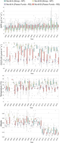
Figure 8. Boxplot of annual values of Albedo, CO₂Flux, GPP, and Temperature for time series 2000 to 2018 in the municipality of Sinop – MT.

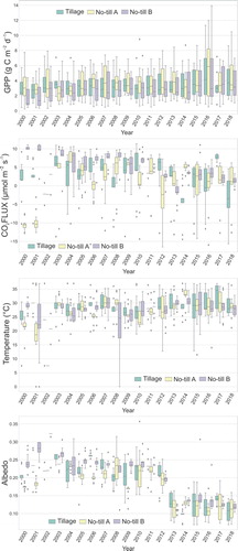
Figure 9. Observed and predicted data for Albedo, CO₂Flux (μmol m⁻² s⁻¹), GPP (g C m⁻² d⁻¹), and Temperature (°C) from January 2000 to December 2018.

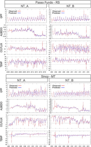
Figure 10. Gross Primary Productivity (GPP) predicted versus observed among 2011 to 2018 years in NT_A and NT_B of Sinop (A and B, respectively), and NT_A and NT_B of Passo Fundo (C and D, respectively).

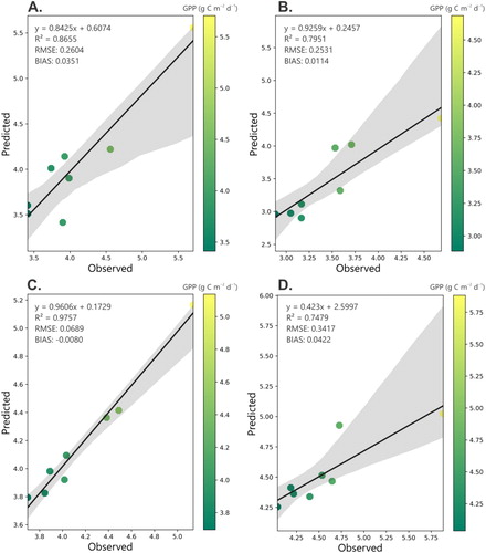
Figure 11. Histogram of each variable on the diagonal, the dispersion by the LOESS curve on the left, and the correlation of values (A – NT_A observed for Passo Fundo; B – NT_A predicted for Passo Fundo; C – NT_B observed for Passo Fundo; D – NT_B predicted for Passo Fundo; E – NT_A observed for Sinop; F – NT_A predicted for Sinop; G – NT_B observed for Sinop; H – NT_B predicted for Sinop) on the right.

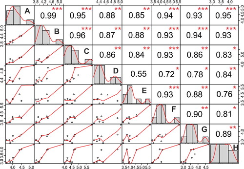
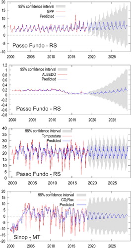
Figure 12. ARIMA model applied to environmental variables: albedo, CO₂Flux, GPP, and temperature for the municipalities of Sinop – MT and Passo Fundo – RS, with a 95% confidence level.

Rouse, J. W., R. H. Hass, J. A. Schell, and D. W. Deering. 1974. “Monitoring Vegetation Systems in the Great Plains with ERTS.” In EARTH RESOURCES TECHNOLOGY SATELLITE SYMPOSIUM, 3., Washington. Proceedings. Washington: NASA, 1974. p. 309–317.

 Google Scholar

Jiang, Z., A. R. Huete, K. Didan, and T. Miura. 2008. “Development of a two-Band Enhanced Vegetation Index Without a Blue Band.” Remote Sensing of Environment 112: 3833–3845.

 Web of Science ®Google Scholar

Qi, J., R. Marsett, P. Heilman, S. Bieden-Bender, S. Moran, D. Goodrich, and M. Weltz. 2002. “Ranges Improves Satellite-Based Information and Land Cover Assessments in Southwest United States.” EOS, Transactions American Geophysical Union 83 (51): 601–606.

 Google Scholar

Marsett, R. C., J. Qi, P. Heilman, S. H. Biedenbender, M. C. Watson, S. Amer, M. Weltz, D. Goodrich, and R. Marsett. 2006. “Remote Sensing for Grassland Management in the Arid Southwest.” Rangeland Ecology & Management 59 (5): 530–540.

 Web of Science ®Google Scholar

Van Deventer, A. P., A. D. Ward, P. H. Gowda, and J. G. Lyon. 1997. “Using Thematic Mapper Data to Identify Contrasting Soil Plains and Tillage Practices.” Photogrammetric Engineering and Remote Sensing 63: 87–93.

 Web of Science ®Google Scholar

Silva, B. B., A. C. Braga, C. C. Braga, L. M. M. Oliveira, S. M. G. L. Montenegro, and B. Barbosa Junior. 2016. “Procedures for Calculation of the Albedo with OLI-Landsat 8 Images: Application to the Brazilian Semi-Arid.” Revista Brasileira de Engenharia Agrícola e Ambiental 20 (1), 3–8. doi:10.1590/1807-1929/agriambi.v20n1p3-8.

 Google Scholar